-
Notifications
You must be signed in to change notification settings - Fork 0
/
Copy pathcross_validation_workshop.Rmd
574 lines (425 loc) · 52.3 KB
/
cross_validation_workshop.Rmd
1
2
3
4
5
6
7
8
9
10
11
12
13
14
15
16
17
18
19
20
21
22
23
24
25
26
27
28
29
30
31
32
33
34
35
36
37
38
39
40
41
42
43
44
45
46
47
48
49
50
51
52
53
54
55
56
57
58
59
60
61
62
63
64
65
66
67
68
69
70
71
72
73
74
75
76
77
78
79
80
81
82
83
84
85
86
87
88
89
90
91
92
93
94
95
96
97
98
99
100
101
102
103
104
105
106
107
108
109
110
111
112
113
114
115
116
117
118
119
120
121
122
123
124
125
126
127
128
129
130
131
132
133
134
135
136
137
138
139
140
141
142
143
144
145
146
147
148
149
150
151
152
153
154
155
156
157
158
159
160
161
162
163
164
165
166
167
168
169
170
171
172
173
174
175
176
177
178
179
180
181
182
183
184
185
186
187
188
189
190
191
192
193
194
195
196
197
198
199
200
201
202
203
204
205
206
207
208
209
210
211
212
213
214
215
216
217
218
219
220
221
222
223
224
225
226
227
228
229
230
231
232
233
234
235
236
237
238
239
240
241
242
243
244
245
246
247
248
249
250
251
252
253
254
255
256
257
258
259
260
261
262
263
264
265
266
267
268
269
270
271
272
273
274
275
276
277
278
279
280
281
282
283
284
285
286
287
288
289
290
291
292
293
294
295
296
297
298
299
300
301
302
303
304
305
306
307
308
309
310
311
312
313
314
315
316
317
318
319
320
321
322
323
324
325
326
327
328
329
330
331
332
333
334
335
336
337
338
339
340
341
342
343
344
345
346
347
348
349
350
351
352
353
354
355
356
357
358
359
360
361
362
363
364
365
366
367
368
369
370
371
372
373
374
375
376
377
378
379
380
381
382
383
384
385
386
387
388
389
390
391
392
393
394
395
396
397
398
399
400
401
402
403
404
405
406
407
408
409
410
411
412
413
414
415
416
417
418
419
420
421
422
423
424
425
426
427
428
429
430
431
432
433
434
435
436
437
438
439
440
441
442
443
444
445
446
447
448
449
450
451
452
453
454
455
456
457
458
459
460
461
462
463
464
465
466
467
468
469
470
471
472
473
474
475
476
477
478
479
480
481
482
483
484
485
486
487
488
489
490
491
492
493
494
495
496
497
498
499
500
501
502
503
504
505
506
507
508
509
510
511
512
513
514
515
516
517
518
519
520
521
522
523
524
525
526
527
528
529
530
531
532
533
534
535
536
537
538
539
540
541
542
543
544
545
546
547
548
549
550
551
552
553
554
555
556
557
558
559
560
561
562
563
564
565
566
567
568
569
570
571
572
573
574
---
title: "Cross-validation workshop"
author: "Mark A. Thornton, Ph. D."
date: "October 11, 2018"
output:
html_notebook:
theme: united
toc: yes
toc_float:
collapsed: false
smooth_scroll: false
---
```{r setup, include=FALSE}
knitr::opts_chunk$set(echo = TRUE)
```
## Introduction to cross-validation
Cross-validation represents a class of powerful procedures for measuring the performance of statistical models. In cross-validation,
a sub-sample of a data set is used to "train" a model - e.g., setting parameters - and this trained model is then used to make predictions
in another, independent subsample of the data. By training and testing in independent data, cross-validation provides an estimate of
the generalization performance of a model - how well it would work when applied to an entirely new data set of the same type. This
helps to minimize the risk of trusting an "overfitted" model which captures a particular data set unrealistically well by capitalizing on chance. This workshop will describe how cross-validation work, with real and artificial examples examined in R.
## Why is cross-validation important?
When fitting a model to a particular data set, it can be hard to tell whether the observed explanatory power of the model (e.g., variance explained, or average error) would generalize to a new, similar data set. Why might a model not generalize from one data set to another? If the model is sufficiently complex, it can capitalize on chance to achieve good performance in the data set to which it is fit. This is known as "overfitting" - let's take a look at the classic example of polynomial regression:
```{r, echo=F, results="hide", include=F}
# load packages
if(!require(MASS)) install.packages("MASS"); require(MASS)
if(!require(glmnet)) install.packages("glmnet"); require(glmnet)
if(!require(e1071)) install.packages("e1071"); require(e1071)
```
```{r fig.height=8, fig.width=8}
# simulate data with quadratic relationship
set.seed(1)
x <- runif(20)-.5
y <- x^2 + rnorm(20,0,.05)
fr <- seq(-.5,.5,by = .001)
# plot
layout(matrix(1:4,2,2,byrow = T))
plot(x,y,main="Raw data",pch=19,cex=1.25)
plot(x,y,main="Linear (y=bx) - underfit",pch=19,cex=1.25)
fit <- lm(y~x)
abline(fit,col="red",lwd=1.5)
sqrt(mean(fit$residuals^2))
plot(x,y,main="Quadratic (y=bx^2) - good fit",pch=19,cex=1.25)
fit <- lm(y~x+I(x^2))
sqrt(mean(fit$residuals^2))
fv <- predict(fit,data.frame(x=fr))
lines(fr,fv, col='red', type='l',lwd=1.5)
plot(x,y,main="High order polynomial (y=bx^9) - overfit",pch=19,cex=1.25)
fit <- lm(y~poly(x,9))
fv <- predict(fit,data.frame(x=fr))
lines(fr,fv, col='red', type='l',lwd=1.5)
sqrt(mean(fit$residuals^2))
```
Here we can see simulated data where the underlying data-generating process is quadratic - the values of y are proportional to x-squared. A linear model completely fails to capture this relationship - what we could call "underfitting" - so we need polynomial regression (with coefficient 2) to achieve a good fit. However, what happens if we make the model too power/complex/highly parameterized? A 9th-degree polynomial appears to fit the data even better, passing very close to almost every point. We can quantify this performance in terms of RMSE - root mean square error. The RMSE of the linear model is .078, quadratic model is .044, and the 9th-order polynomial is .03 (smaller RMSE is better). However, this model is overfitted to the particular data in question, as we can see when we examine new data generated by the same process, as illustrated below.
```{r fig.height=4, fig.width=8}
set.seed(2)
x2 <- runif(20)-.5
y2 <- x2^2 + rnorm(20,0,.05)
layout(matrix(1:2,1,2,byrow = T))
plot(x,y,main="Quadratic (y=bx^2)",pch=19,cex=1.25)
fit <- lm(y~x+I(x^2))
fv <- predict(fit,data.frame(x=fr))
x2f <- predict(fit,data.frame(x=x2))
sqrt(mean((x2f-y2)^2))
lines(fr,fv, col='red', type='l',lwd=1.5)
points(x2,y2,col="blue",pch=19,cex=1.25)
segments(x2,y2,x2,x2f,col="blue")
plot(x,y,main="High order polynomial (y=bx^9)",pch=19,cex=1.25)
fit <- lm(y~poly(x,9))
fv <- predict(fit,data.frame(x=fr))
x2f <- predict(fit,data.frame(x=x2))
sqrt(mean((x2f-y2)^2))
lines(fr,fv, col='red', type='l',lwd=1.5)
points(x2,y2,col="blue",pch=19,cex=1.25)
segments(x2,y2,x2,x2f,col="blue")
```
The new data points here are illustrated in blue, and the errors made by the model are illustrated by the blue lines between the red model fit and the new data points. Both models make errors, but the simpler quadratic model now makes smaller errors (RMSE = .064) than the 9th-degree polynomial (RMSE = .082). This reversal illustrates the unrealistic high performance promised by the more complex model when fitted without out-of-sample validation.
So how can we defend against cross-validation? We cannot simply always choose the simplest model, because - as have seen in the case of the linear fit above - it may not help us explain our data, or predict new data, at all. One way to reduce overfitting is to increase the size of your sample - you can see this illustrated below.
```{r fig.height=8, fig.width=8}
set.seed(1)
layout(matrix(1:4,2,2,byrow = T))
fr <- seq(-.5,.5,by = .001)
x <- runif(20)-.5
y <- x^2 + rnorm(20,0,.05)
plot(x,y,main="N = 20",pch=19,cex=1)
fit <- lm(y~x+I(x^2))
fv <- predict(fit,data.frame(x=fr))
lines(fr,fv, col='blue', type='l',lwd=3)
fit <- lm(y~poly(x,9))
fv <- predict(fit,data.frame(x=fr))
lines(fr,fv, col='red', type='l',lwd=3)
x <- runif(100)-.5
y <- x^2 + rnorm(100,0,.05)
plot(x,y,main="N = 100",pch=19,cex=1)
fit <- lm(y~x+I(x^2))
fv <- predict(fit,data.frame(x=fr))
lines(fr,fv, col='blue', type='l',lwd=3)
fit <- lm(y~poly(x,9))
fv <- predict(fit,data.frame(x=fr))
lines(fr,fv, col='red', type='l',lwd=3)
x <- runif(500)-.5
y <- x^2 + rnorm(500,0,.05)
plot(x,y,main="N = 500",pch=19,cex=1)
fit <- lm(y~x+I(x^2))
fv <- predict(fit,data.frame(x=fr))
lines(fr,fv, col='blue', type='l',lwd=3)
fit <- lm(y~poly(x,9))
fv <- predict(fit,data.frame(x=fr))
lines(fr,fv, col='red', type='l',lwd=3)
x <- runif(2500)-.5
y <- x^2 + rnorm(2500,0,.05)
plot(x,y,main="N = 2500",pch=19,cex=1)
fit <- lm(y~x+I(x^2))
fv <- predict(fit,data.frame(x=fr))
lines(fr,fv, col='blue', type='l',lwd=3)
fit <- lm(y~poly(x,9))
fv <- predict(fit,data.frame(x=fr))
lines(fr,fv, col='red', type='l',lwd=3)
```
As you can see, as the sample size increases, the overly-complex 9th-degree polynomial gradually converges on the simpler quadratic fit which better explains the data-generating process. However, while increasing one's sample size is generally desirable (all-else-equal) it is often impractical to do so beyond a certain point due to practical constraints such as time and money. How can we know whether our model is disastrously overfitting our data with the largest sample we can afford to collect? This is where cross-validation comes in.
## Basic forms of cross-validation
Out-of-sample model validation is a way to estimate the generalization performance of a statistical model. The simplest form of validation is to train a model on one data set, and then test it on another, independent, data set. So where does the "cross" in cross-validation come from? In cross-validation, this validation procedure is repeated, treating each independent data set (or sample from within a single data set) as both the training and the testing sequence in turn.
### Split-half cross-validation
The simplest form of cross-validation is two divide the data set into two even halves. The model is first trained on half one, and then tested on half two. Then the process is reversed, and the model is trained on half two and tested on half one. This produces two performance values (RMSEs, correlations, etc.) that are typically averaged together to produce a single estimate of model performance. This procedure is known as split-half cross-validation.
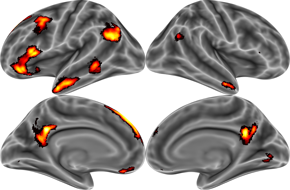
Let's try it out, this time using some real data. These data come from [Thornton and Mitchell, 2017, Cerebral Cortex](http://markallenthornton.com/cv/Thornton&Mitchell_CC_2017.pdf), and fMRI-based investigation of the neural organization of person knowledge. In the MRI scanner, participants repeatedly made a variety of inferences about a set of 60 famous target people (e.g., "How much would Bill Nye like to learn karate?"). For the purposes of today's class, I've extracted the average brain activity associated with each target person within the social brain network (see below).
Our goal in this instance will be to try to predict the average brain activity across this entire network, based on ratings of the psychological traits of the target people (e.g., warmth and competence) provided by a separate group of raters. To this end, we'll perform a split-half with respect to the target people, to measure how well our model can generalize from one set of famous target people to another.
```{r}
# load fMRI data
bdat <- read.csv("brain_data.csv")
# average across participants (we'll come back to this later)
bmeans <- rowMeans(bdat)
# load rating data
dat <- read.csv("ratings.csv")
rat <- as.matrix(dat[,2:14])
rownames(rat)<-dat$name
# perform split-half
# normally we'd split halves randomly, but the targets are already in an arbitrary order, so we'll just take the 1st 30 and last 30
half1.brain <- bmeans[1:30]
half1.ratings <- rat[1:30,]
half2.brain <- bmeans[31:60]
half2.ratings <- rat[31:60,]
# train ridge regression
trainperf <- rep(NA,2)
cvfit <- cv.glmnet(half1.ratings,half1.brain,alpha=0,lambda=10^seq(-3,3,by=1))
# compute predictions in other half of data
predvals <- predict(cvfit$glmnet.fit,s=cvfit$lambda.min,newx=half2.ratings)
# evaluate performance via correlation
perf <- rep(NA,2)
perf[1] <- cor(predvals,half2.brain)
# repeat, switching halves
cvfit <- cv.glmnet(half2.ratings,half2.brain,alpha=0,lambda=10^seq(-3,3,by=1))
predvals <- predict(cvfit$glmnet.fit,s=cvfit$lambda.min,newx=half1.ratings)
perf[2] <- cor(predvals,half1.brain)
# mean performance (r)
mean(perf)
```
As you can see, in this cross-validation, we're able to predict brain activity out-of-sample moderately well, with an average correlation between cross-validation predictions and actual activity of r = .51. Yay!
Split-half cross-validation is simple to execute, making it moderately popular. However, it has an important downside: as we saw earlier, models tend to do better at avoiding overfitting when they're trained on larger data sets. However, with split-half cross-validation, we're holding fully half of our data in reserve for testing, meaning that we only get to use half for training. If we have a small dataset, as we do here, then that can really hurt us. Is there anything to be done?
### K-fold cross-validation
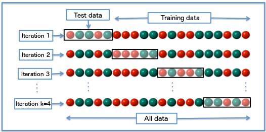
The k-fold scheme is a form of cross-validation which is often preferable to split-half. It consists of splitting the data into an arbitrary number of parts (or "folds") - that's the "k" in k-fold. On each of k iterations, the model is then trained on (k-1) parts of the data (so if k = 4, 3/4ths) and tested on the remaining part. The cross-validation procedure cycles through the different parts, treating each of the k-folds as the test set in turn (see illustration below).
k-fold cross-validation has the advantage of using more of the total data set as training. How much depends on what value we choose for k, with larger k values meaning more training data: training data is (k-1)/k of the total data. There are a lot of papers discussing ideal values for k, and how to choose them based on factors such as the number of observations in your data, and how long your model takes to train. That's beyond the scope of today's tutorial, but in most cases you'll probably do pretty well setting a k somewhere between 4 and 10. Let's repeat the analysis above using 4-fold cross-validation instead of split-half.
```{r}
# There are probably dozens of existing functions in existing R packages that allow you to define indics for cross-validation.
# I create this one from scratch so that you can see the basic principle.
cvinds = function(n,k){
inds <- rep(1:k,ceiling(n/k))
inds <- sample(inds)[1:n]
return(inds)
}
# create indices
set.seed(1)
k <- 4
n <- dim(dat)[1]
inds <- cvinds(n,k)
# loop through training and testing
perf <- rep(NA,k)
for (i in 1:k){
sel <- inds == i
cvfit <- cv.glmnet(rat[!sel,],bmeans[!sel],alpha=0,lambda=10^seq(-3,3,by=1))
predvals <- predict(cvfit$glmnet.fit,s=cvfit$lambda.min,newx=rat[sel,])
perf[i] <- cor(predvals,bmeans[sel])
}
mean(perf)
```
We can see that the average performance is now a bit higher than it was in the split-half version. Note that the precise value of the performance here depends on the random seed. Some "unlucky" 4-fold splits might produce lower performance, while "luckier" ones might produce higher. When you have a small data set, it is often a good idea to run the analysis multiple times and average across different random seeds to get a more stable estimate. It's also very important to set the random seed at the beginning of the analysis to ensure reproducibility.
So, why might performance with 4-fold cross-validation be better than with split-half? Just as we saw in our overfitting example, more data can result in more generalizable parameters for a model. When you see that model performance improves as a function of increasing the size of the training set, this suggest that your model needs more data to achieve its most generalizable fit. Examining the curve which relates sample size to model performance can help you do something analogous to a power analysis: choose how large of a sample you need. At a certain point, adding more data won't improve performance any more. Where this point lies will depend on numerous factors, including the signal-to-noise ratio in the data, how heterpgenous/variable your data are, and how complex a model you need. Also, bear in mind that you should not compare different models assessed using different cross-validation schemes because any differences between them might result from the differences in the procedure rather than differences between the models.
### Leave-one-out cross-validation
Some of you may already have realized that split-half cross-validation is actually just a special case of k-fold cross-validation, where k = 2. If having more training data generally improves model performance, than perhaps you're now thinking about the other extreme: how big can we make k? The absolute limit on k is k = n, where n is the number of observations in the data set. This special case also has a special name: leave-one-out (LOO) cross-validation. In LOO, each observation is left out in turn. A model is fit on all of the other data, and then that model is applied to predict the one left-out point.
LOO has a couple of features which make it attractive. First, it maximizes the size of the training set, given the overall size of a data set. Second, it has only one unique solution: since there's only one way to leave each individual point out, there's no need for a random split of the data into k parts.
However, LOO also has some drawbacks, which are less obvious but no less serious. First, LOO is slow: it requires fitting the model more times than any other scheme, and the model fitting takes longer each time because the most data possible is used. With small data sets this won't make much difference, it can be extremely important when larger data sets are considered. Second, LOO is unstable. Although it produces a unique value within a given data set, research suggests that it is counterintuitively less replicable across data sets than k-fold with moderate k values. Third, LOO can limit the metrics you can use for assessing accuracy. For instance, calculating a correlation requires multiple points, but only a single value is predicted on each iteration of LOO. However, there are ways to circumvent this limitation, as we'll see below. Finally, LOO can lead to or exacerbate some truly bizarre performance, as we'll see in the case below:
```{r fig.height=6, fig.width=6}
# Here we return to simulated rather than real data. The Xs and y here are simulated to be unrelated to each other.
set.seed(1)
x <- data.frame(matrix(rnorm(100),50,2))
y <- rnorm(50)
# fit (un-cross-validated regression)
summary(lm(y~as.matrix(x)))
# Here we conduct a simple multiple regression with 2 Xs and 1 y, using a LOO CV scheme
pred <- rep(NA,50)
for (i in 1:50){
curx <- x[-i,]
fit <- lm(y[-i]~as.matrix(curx))
curx <- x[i,]
pred[i]<-predict(fit,curx)
}
# evaluate performance
plot(pred,y,xlab="predicted",ylab="actual",pch=19)
```
In the example above, we generate a model based on random normal data, with predictors (x) and one dependent variable (y). As you would expect, when you fit this model using a standard OLS regression (without cross-validation) the R-squared of the model is almost exactly 0. We should thus expect change performance (a correlation of 0) in our cross-validated version of the same analysis, right? We run that model, using a work-around to evaluate the correlation between predictions actual y-values, but observe something dramatically different. We see a large negative(!!!) correlation between predictor and predicted. Genuinely negative/below-chance performance scores are possible in cross-validation, in a process called "[anti-learning](http://www.cyberneum.de/fileadmin/user_upload/files/publications/alt_05_[0].pdf)." However, anti-learning is extremely rare in practice, and definitely not present in the current simulated data set.
What's actually going wrong here is something more insidious. Every time you take one data point out, it shifts the mean of the sample in the opposite direction with respect to the overall sample mean. For example, in this data set the mean of the DV is ~0, so if LOO removes a point with a score of 1, then the mean will move "down" (i.e., to a more negative value). Because the sample is small, this shift is nontrivial. Since the two regressors are unrelated to the dependent variable, most of the "prediction" that happens in this model is down to the intercept of the regression. And what does that intercept model? The mean. Since the mean constantly moves away from the left-out value, LOO cross-validation is actually manufacturing a spurious negative correlation between predicted and observed values. The situation illustrated here is about as bad as it can be: few data points, few predictors, and zero actual correlation. However, you'll notice that it is not too dissimilar from the real data we examined above, and it is by no means unrealistic for much psych/neuro data. You can read more about this particular issue on Russ Poldrack's blog [here](http://www.russpoldrack.org/2012/12/the-perils-of-leave-one-out.html).
All-in-all, for reasons including the one above, leave-one-out cross-validation is rarely the best choice for analyzing a data set. It's often not too deleterious either, and remains generally popular, but your default cross-validation scheme should probably be something more like k=4-10 fold cross-validation.
### Advanced cross-validation schemes
Most cross-validations you'll see in the literature will consist of one of the three schemes we've seen above. Sometimes, these will be augmented by particular features of the data set in question. For example, in fMRI, where data is collected over the course of multiple runs, you will often see "leave-one-(run)-out" cross-validation. Since each run consists of many data points, this can be thought of LOO at the level of runs, or a particular way of doing k-fold cross-validation (where k = the number of runs, and data points are not sorted randomly into the folds).
However, there are other, more sophisticated types of cross-validation. In fact, we've already seen one, though it probably wasn't obvious. In the analysis of neural data, we used a ridge regression. Ridge regression is very similar to standard OLS regression, but it has a regularization parameter (lambda) which is used to help deal with multi-collinearity and the curse of dimensionality. Ridge regression's lambda is an example of a "hyperparameter." Hyperparameters control how a model is fit, rather than describing its ultimate fit. For example, in ridge regression, the hyperparameter lambda influences how much the regression coefficients (regular old parameters) are "shrunk" towards zero. Unfortunately, it's hard to know what the best hyperparameters are without looking at the data. Thus, in the ridge regression examples above, we first use the "cv.glmnet" function to conduct what is known as a "grid search" - as systematic trial of different hyperparameters, to see which one works best. By work best, in this case we mean produces the smallest error in a k-fold cross-validation. Thus, those analyses are actually multi-step cross-validations in which the hyperparameters are first fit through k-fold cross-validation within the training set, and then the entire training set is used to predict the test set.
Overfitting can happen at the level of model fitting or hyper parameter selection, and this is why we sometimes need multi-step cross-validation. However, overfitting can also happen at what one might call the "cognitive" or "researcher" level. That is, if I try many different models and compare their fit, choosing the better ones or tweaking them to get better performance, I may see real improvement in my model performance, but I am also liable to capitalize on chance. This process is analogous to p-hacking in the null-hypothesis significance testing framework. Although cross-validation is a powerful technique, it alone cannot save us from ourselves: even cross-validated model performance is subject to this sort of "hacking". The machine learning world has come to realize this as a problem, as several papers in different fields of research have demonstrated that existing algorithms are greatly overfit to certain canonical test sets. Note that this goes beyond the normal practice of p-hacking (which is usually thought to happen within a single person or research group) to the level of an entire field. You could thus think of it as distributed p-hacking. This problem hasn't affected psychology to the same extent because everyone is out collecting their own data sets, rather than referring to a few canonical validation data sets. However, as large-scale psychology projects like Many Labs become common, we may need to think about this issue in more detail.
What can you do to protect yourself from cognitive/researcher-level overfitting? The common practice is to hold out a subsample of the data from the very beginning. With the rest of the data, you can analyze and tweak and fiddle to your heart's content (of course, using cross-validation to get more generalizable performance estimates in each individual case). However, at the end of the day, you then run your favorite models on the as-yet untouched hold-out set. Performance in the hold-out set, rather than in the rest of the data, is thus used as a basis for inference, and no further tweaking is allowed (or at least, fully trusted).
#### Bi-cross-validation
One particularly sophisticated form of cross-validation which is often relevant to psychologists is [bi-cross-validation](https://arxiv.org/pdf/0908.2062.pdf) for principal component analysis (PCA). PCA is a popular technique for dimensionality reduction in psychology. One of the biggest challenges in PCA is to identify the appropriate number of instrinsic/true/latent dimensions in a dataset. There many parametric and quasi-parametric approaches for selecting the PC number, ranging from the classic but often misleading Kaiser criterion, to sophisticated modern alternatives like parallel analysis and Velicer's MAP. However, virtually all of the existing techniques carry certain assumptions, which are often violated by real data. This makes cross-validation a promising solution.
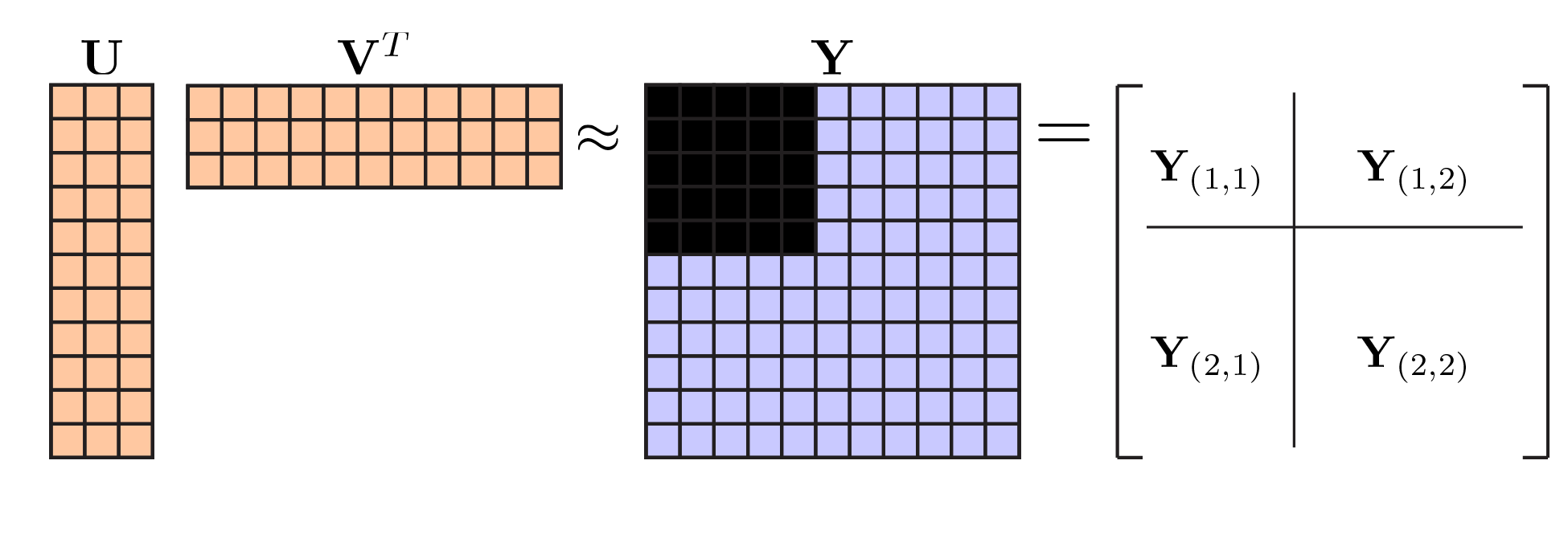
As we've previously discussed, the key feature necessary for valid cross-validation is independence of the training and test sets. The
training set should have no information about the test set. However, this because trickier in PCA, because there are two types of "information" the model might have: information about the observations, and information about the variables. The way bi-cross-validation works is to cross-validate in two direction at the same time. Let's see how it works:
```{r fig.height=6, fig.width=6}
# Let's begin by simulating data with 50 nominal dimensions, but only 5 underlying latent dimensions:
set.seed(1)
x <- scale(matrix(rnorm(5000),1000,50) + matrix(rnorm(50000),1000,50))
# There's so much "signal" in this toy example that we don't really need a fancy technique to find the right answer.
# Simply examining the scree plot is sufficient:
pcares <- prcomp(x)
plot(1:50,pcares$sdev^2/50,xlab="PC #",ylab="% variance explained",pch=19,type="o")
# The first step in bi-cross-validation is to perform a PCA on 1/2 the variables and 1/2 the observations
initpca <- princomp(x[501:1000,26:50])
# Next, we compute a PCA-regression from the scores of this PCA to other 1/2 of variables
pcrfit <- lm(x[501:1000,1:25]~initpca$scores)
# In the third step, we create PCA scores in the other 1/2 of observations (but initial half of variables)
weimat <- lm(x[501:1000,26:50]~initpca$scores)$coefficients[2:26,1:25] # compute weight matrix
pc2 <- x[1:500,26:50] %*% weimat
# Finally, we use the PCR weights from the second step, in combination with the PC scores from the third step,
# to predict the variable values in the final piece of as-yet untouched data.
perf <- rep(NA,25)
for (i in 1:25){
predvals <- as.matrix(pc2[,1:i]) %*% pcrfit$coefficients[1:i,]
perf[i] <- sqrt(mean((x[1:500,1:25]-predvals)^2))
}
plot(perf,xlab="PC #",ylab="RMSE",type="o",pch=19)
```
As you can see, the model achieves minimum error at 5 PCs, precisely as it should. In a real analysis, we would want to repeat this analysis across multiple training and tests sets, but since these are toy data, that's not really necessary.
## Model performance, comparison, and selection
It goes without saying that there are many different types of statistical model, ranging from tried-and-true standards like linear regression to state-of-the-art techniques from deep learning. Discussion of such models and their differences is largely beyond the scope of this tutorial. The value of cross-validation is that it can be applied to any of them, to assess their performance and ability to generalize. Moreover, it allows us to compare models with one another on a common performance metric.
### Model performance metrics
There are a number of different ways of measuring model performance in the context of cross-validation. There are advantages and disadvantages to the different measures, so it's important to choose the right one for the problem at hand, or even better, examine multiple measures. The first and most important question you need to think about when choosing performance metrics is the scale level of your outcome variable. The performance measures for regression problems - in which the dependent variable is continuous/metric - are completely non-overlapping with the metrics available for classification problems - in which the outcomes are categorical/nominal.
#### Regression metrics for continuous DVs
We've already seen examples of two of the most prominent model performance metrics for regression problems: root mean square error (RMSE) and correlation (R). Let's talk about these metrics a little more. RMSE is a useful measure for assessing the performance of models in which you predict real-world outcomes. This is because RMSE provides a measure of model performance that is on the same scale as your dependent variable. So if you're predicting the amount of money a movie will gross, your RMSE will be expressed in terms of dollars ($). It's also fairly easy to interpret RMSE: it's effectively the average error that your model will make.
Correlations are also a useful metric, for precisely the opposite reason: they are standardized and scale-free. When using correlation as your performance metric, it doesn't matter whether your units are dollars, seconds, meters, or megabytes: you will still end up with a value on the interval [-1,1]. RMSE values can be standardized, usually by diving them by their range, but they're still a bit less intuitive to interpret then correlations. However, the standardization of correlations can encourage dangerous comparisons. Comparing one model, with one cross-validation scheme, predicting one variable, to another model, using another cross-validation scheme, predicting another variable, will rarely yield meaningful information and can be quite deceptive. In passing, I'll also mention that R-squared (or % of variance explained) is another common performance metric that is closely related to correlation (simply being the square of R).
#### Classification metrics for categorical DVs
A completely different set of metrics are used to assess the performance of classification models with categorial outcomes. In these cases, there are several important measures:
1. Accuracy: this is simply how often your model predicts the correct categorical value in the test set.
2. Sensitivity (aka true positive rate or recall): % of category X correctly labeled as category X
3. Specificity (aka true negative rate or selectivity): % of "not X" correctly labeled as "not X"
4. Positive predictive value (aka precision): % of cases labeled X that are actually X
5. Negative predictive value: % of cases labeled "not X" that are actually "not X"
There are several other related values, such as the false positive and negative rates (fall-out and miss rate, respectively), as well as the false discovery rate and the false omission rate. All of these metrics are related to one another, and some are fully redundant from a mathematical point of view. There's an excellent table available [here](https://en.wikipedia.org/wiki/Positive_and_negative_predictive_values#Relationship) that illustrations the relations between them. Which measures you want to focus on probably depends on your research problem. For example, in practical problems such as disease-detection, it may be better to focus on sensitivity, to avoid missing any case of a disease, and on positive predictive value, to avoid over-diagnosis.
For the moment, however, let's work through an example problem. This example comes from my wine research, rather than psychology/neuroscience. There are many different varieties of microorganisms that can grow in wine, some more desirable than others. The main fermentation yeast is called Saccharomyces cerevisiae (shown below), but there are many other yeast and bacteria which may help (or more usually, spoil) the winemaking process. In collaboration with my parents, I developed a chemometric approach to classifying three different species of common wine bacteria based on their Raman spectroscopy spectra (you can read more [here](http://markallenthornton.com/blog/wine-raman-classification/)).

The example we'll consider uses data from that study. We'll use a split-half approach to classify several hundred bacteria samples into one of three genuses. The model we're using a bit more sophisticated - a support vector machine classifier - but you don't need to worry about the details of how it works for our present purposes.
```{r}
# load bacteria data
bact <- read.csv("bacteria.csv")
# generate C-V indices
set.seed(1)
inds <- cvinds(dim(bact)[1],2)
# train linear SVM on half of the data
svmfit <- svm(bact[inds==1,2:3202],bact$genus[inds==1],kernel = "linear")
# predict labels in other half of datasvm
predvals <- predict(svmfit,bact[inds==2,2:3202])
# tabulate actual vs predicted
ta <- table(bact$genus[inds==2],predvals)
ta
```
The table you see above reflects the performance of the classifier. All of the specific indices of model performance mentioned earlier can be calculated by summing and dividing by various components of this table. Let's see how!
```{r}
# 1. accuracy: diagonal over total
sum(diag(ta))/sum(ta)
# 2. sensitivity: diagonal over row totals
diag(ta)/rowSums(ta)
# 3. specificity:
(sum(ta)-(rowSums(ta)+colSums(ta)-diag(ta)))/(sum(ta)-rowSums(ta))
# 4. positive predictive value: diagonal over column totals
diag(ta)/colSums(ta)
# 5. negative predictive value:
(sum(ta)-(rowSums(ta)+colSums(ta)-diag(ta)))/(sum(ta)-colSums(ta))
```
As you can see, accuracy requires counting all true positive and true negatives, and thus can only be calculated with respect to the full classification problem. In contrast, the other measures we detailed can each be calculated separately for each condition. Note that there is considerable variation in these performance metrics, both across the different bacteria and across the different metrics.
It's also worth noting that the performance here is worse than what we report in the published paper. This is because we're simplifying the problem by assuming each genus of bacteria is homogeneous. In reality, each is composed of several many different strains. Sometimes there's more variance between strains within a genus, than between different genuses, in terms of Raman spectra. Thus in the paper we did better at the genus level by leveraging information at the strain level.
### Model comparison
How can we tell whether one model is better than another? This is a crucial question, since incremental improvement in science requires us to pit competing models against one another. There are a number of statistics for model comparison which you might be familiar with from more traditional data analyses. These include R-squared and adjusted R-squared, Akaike's Information Criterion (AIC) and Bayesian Information Criterion (BIC), and likelihood ratio tests. These statistics are useful, and arguably underused, but they have a number of disadvantages relative to cross-validated model performance measures. Some, like (unadjusted) R-squared, don't properly adjust for model complexity. For example, in a multiple regression, the R-squared will continue to rise monotonically as you add more predictors, even if those predictors are just random noise. Other model comparison statistics can only be computed in very specific situations. For instance, likelihood ratio tests can only compare nested models. More generally, most statistics - even AIC and BIC - have more extensive assumptions built into them than cross-validation. This makes cross-validation an exceptionally widely applicable way to compare models.
Let's return to our person perception fMRI data to conduct some model comparison. Below we'll use 5-fold cross-validation to compare two models of person perception: the stereotype content model (warmth and competence) and the agency and experience model of mind perception.
```{r}
# create indices
set.seed(1)
k <- 5
inds <- cvinds(60,k)
# loop through folds
perf <- matrix(NA,k,2)
colnames(perf)<-c("scm","a&e")
for (i in 1:k){
# slice folds
sel <- inds==i
y <- bmeans[!sel]
# fit and evaluate scm
x <- rat[!sel,c(13,4)]
fit <- lm(y~x)
x <- rat[sel,c(13,4)]
pred <- predict(fit,data.frame(x))
perf[i,1]<-sqrt(mean((pred-bmeans[sel])^2))
# fit and evaluate a&e
x <- rat[!sel,c(1,7)]
fit <- lm(y~x)
x <- rat[sel,c(1,7)]
pred <- predict(fit,data.frame(x))
perf[i,2]<-sqrt(mean((pred-bmeans[sel])^2))
}
colMeans(perf)
```
As you can see, the perform of the stereotype content model (scm) is slightly better than the perform of the agency and experience model (a&e). Remember that we are looking at RMSE here, and lower error mean better performance. This is as simple as model comparison gets with cross-validation. However, by iterating over this simple operation, you can also perform more complicated tasks like model selection. For example, we could compare every possible combination of the trait dimensions in the current data set to choose the best one (a more modern way to do this might be through LASSO regression). Such model selection can have a dramatic effect on the performance of predictive models. However, it is important to remember to always separate your test and training set. In the case of model selection, simply considering so many models can bias estimates of the best model's performance. Thus a subset of the data should be held out to get an unbiased estimates of how well the best model performs.
### Null hypothesis significance testing
You might have noticed in the previous section that the numerical difference between the performances of the two models was very small - less than 0.02. How can we know whether such a difference is meaningful? One response might be to ask how we know that any statistical difference is important? There are multiple ways of assessing such a thing, ranging from standardized effect size measures, to implications for real world problems. In psychology and neuroscience, you may often be asked to put a p-value on things before people believe it. Doing so is not always particularly helpful, but it is possible. How? Let's start with what not to do:
#### 1. Do not treat "folds" of a cross-validation as independent!
It might be tempting to treat each "fold" in a cross-validation procedure as an independent estimate, and do something like a t-test on performance across folds. Unfortunately, this procedure is fundamentally flawed because the folds are not independent. Sure, the tests sets are each independent of the other test sets. However, the training sets are all highly overlapping with all of the other training sets! As a result, applying a parametric test across folds violates the independence assumption common to most such tests, and will yield very misleading p-values. It's also worth pointing out that the number of folds is something the analyst chooses, but it would determine the degrees of freedom of a parametric test across folds. There is something deeply wrong with any procedure that allows the analyst to manufacture their own degrees of freedom in this way.
#### 2. Do not perform binomial tests on cross-validated accuracy!
I sometimes see people reason along the following lines: accuracy for classification is a binary value - right or wrong. Therefore, I can apply a binomial test to cross-validated accuracies to get p-values associated with a certain set of predictions. This obviously a non-starter when one is working with regression rather than classification, but it is also problematic for classification. Again, the reason is a violation of the independence assumption. If you did a single split-half, and then computed a binomial test on the accuracy in the test half, this would not be too wrong (though less than ideal, in multiclass cases). However, if one then completed the "cross" in cross-validation (reversing the training and testing halves) to generate predictions for the first half, and then computed a binomial test across ALL observations, this would again violate the independence assumption of the test, for the same reason as #1.
#### NHST with cross-validation: Permutation testing
The most common way to obtain valid p-values with cross-validation is through permutation testing. First, one computes the actual performance of the model, on whatever metric one chooses. Next, one repeatedly re-computes this model performance statistic on randomized data. There are multiple possible permutation schemes, but one of the simplest is shown below: shuffling the DV (numeric outcome/labels) with respect to the entire predictor matrix. In this case, we will return to the question of whether the two model of person perception examined above perform significantly differently from each other.
```{r}
orig.perf <- colMeans(perf)
perfdiff <- orig.perf[2]-orig.perf[1]
# here we perform the permutation
# note that most of the code is the same as in the original case
# however, we wrap the innner k-fold in an outer permutation loop
set.seed(1)
nperf <- 1000
permperfdiff <- rep(NA,nperf)
for (p in 1:nperf){
pbmeans <- sample(bmeans)
perf <- matrix(NA,k,2)
for (i in 1:k){
# slice folds
sel <- inds==i
y <- pbmeans[!sel]
# fit and evaluate scm
x <- rat[!sel,c(13,4)]
fit <- lm(y~x)
x <- rat[sel,c(13,4)]
pred <- predict(fit,data.frame(x))
perf[i,1]<-sqrt(mean((pred-pbmeans[sel])^2))
# fit and evaluate a&e
x <- rat[!sel,c(1,7)]
fit <- lm(y~x)
x <- rat[sel,c(1,7)]
pred <- predict(fit,data.frame(x))
perf[i,2]<-sqrt(mean((pred-pbmeans[sel])^2))
}
permperfdiff[p]<-colMeans(perf)[2]-colMeans(perf)[1]
}
hist(permperfdiff,20,col="grey80",title="Distribution of permuted performance")
abline(v=perfdiff,col="red",lwd=2)
mean(abs(permperfdiff)>perfdiff)
```
Above you can see the results of the permutation test. The grey histogram illustrates the empirical null distribution. Even if you're not interested in statistical significance, it can be helpful to generate such a null distribution to ensure there's nothing wrong with your code that's allowing your model to perform above chance on random data. The red line indicates the difference in model performance we actually observed. Since we want a 2-sided test, we take the absolute value of the permutation distribution, and then calculate the fraction of those values that are greater than the unpermuted effect. In this case, that corresponds to p = .004, indicating that the stereotype content model significantly outperformed the agency and experience model in predicting overall social brain network activation to mentalizing about different famous people.
You might be wandering how many permutations you need to run. This depends on two factors: how precisely you need to estimate your p-values, and how much time it takes to run a permutation. Typically numbers include 1000, 5000, and 5000. However, if you need to estimate very small p-values precisely, then you made need to run more. Running as many as you have time for (however you define that) is not bad rule of thumb.
In this analysis, and all previous analyses of the person perception data, we have been conducting what amounts to an item-analysis. That is, we have collapsed across participants (via averaging) prior to fitting and evaluating our models. Thus, the p-value reported above indicates a fixed effect analysis with respect to participant: we cannot necessarily expect this same result in a new sample, unless there are no meaningful individual differences in social perception (a possibility which seems rather unlikely, a priori). To obtain random effects p-values, you might imagine that you could perform this cross-validated model comparison separately in each participant, and then compare the difference to 0 across participants using a t-test. Unfortunately, this intuitive solution also yields a fixed effect analysis with respect to participants. Even performing the permutation testing within each participant is not enough - the results of individual subject permutation have to be combined using a second-level bootstrapping procedure to obtain something akin to a random effects p-value. The details are beyond the present workshop, but you can read more [here](https://arxiv.org/abs/1512.00810).
## Specific generalization: validation across boundaries
Cross-validation is all about measuring the generalizable performance of predictive models. However, just what are we generalizing over? That depends on how one structures the validation process. Validating model performance across various different boundaries in your data set can prove highly informative with respect to just how generalizable your results really are, and with respect to what.
Let's consider the person perception data we've been working with so far. At the beginning, we actually loaded in data from 29 different participants. However, as discussed in the last paragraph, ever since we've been working with data which was collapsed with respect to participant. Here we will undo that, and work with the full data set. Doing so allows us to do something really interesting: examine how well a model generalizes across participants, across famous target people, or across neither. We'll keep things simple by examining just one model: in this case, the stereotype content model, since it "won" the model comparison in the previous section. We'll also keep things simple by just doing a single split-half, rather than a more complex k-fold.
```{r}
# "stack" the dataset into long form
allbrains <- as.numeric(as.matrix(bdat))
nobs <- length(allbrains)
scm <- matrix(rat[,c(13,4)],nobs,2)
# define train/test function
tteval <- function(x,y,inds){
yc <- y[inds]
xc <- x[inds,]
fit <- lm(yc~xc)
xc <- x[!inds,]
predvals <- predict(fit,data.frame(xc))
perfc <- rep(NA,2)
perfc[1] <- cor(predvals,y[!inds])
yc <- y[!inds]
fit <- lm(yc~xc)
xc <- x[inds,]
predvals <- predict(fit,data.frame(xc))
perfc[2] <- cor(predvals,y[inds])
return(mean(perfc))
}
# we'll loop several different split-halves, and average across them, to get more stable estimates
set.seed(1)
ns <- 100
perf <- matrix(NA,ns,3)
colnames(perf)<-c("all","part","targ")
for (i in 1:ns){
# 1st, a generic split-half that doesn't use any participant/target info
sp.all <- cvinds(nobs,2)==1
perf[i,1] <- tteval(scm,allbrains,sp.all)
# 2nd, we need a split-half of participants
sp.part <- rep(sample(rep(c(T,F),15))[1:29],each=60)
perf[i,2] <-tteval(scm,allbrains,sp.part)
# 3rd, a split-half by target person
sp.targ <- rep(sample(rep(c(T,F),30)),29)
perf[i,3] <-tteval(scm,allbrains,sp.targ)
# we'll start with the random split-half
}
colMeans(perf)
```
There are a few things you might notice about these results. One is that all of the values are much smaller in magnitude than those we saw when working with the same data earlier in the workshop. This is interesting, but not really directly related to cross-validation. It's an effect of correlation attenuation: the less reliable your measures, the lower the meaningful correlation you can expect to observe between them. Earlier we were working with data that averaged across participants, and that averaging boosted the reliability of the resulting composite (just like averaging items in a scale). However, when we returned to the individual participant level in this example, our performance took an (apparent) hit as a result.
The more relevant thing you might notice about these data is that the performances for the participant-respecting split-half, and the target-respecting split-half, are substantially lower than the performance of the fully random split-half across all of the data. Why might this be the case? In each case the training model had access to the same raw quantity of data (i.e., half of it), so this has to be about data quality instead. In the "all" cross-validation, the training data contained information about all participants and all target people, so it really only had to generalize to new data within these conditions. In contrast, the "part" cross-validation training model knew about all target people, but only half of the participants, so it had to generalize to a new sample of participants from the same population. Since these participants were not perfectly identical to those in training set, the model suffered as a result. Similarly, in the "targ" cross-validation, the training model knew about all participants, but only about half of the target people. Again, the training and test sets were sufficiently similar to permit some generalization, but only with a reduction in predictive performance.
We can see that both of these "boundaries" in the data - participant and target person - reduced the performance of the model substantially: more than half relative to the completely random split-half. If we wanted to, we could also combine these two boundaries, forcing the model to generalize across both participants and targets. This would require a different cross-validation scheme, because two non-overlapping halves of the data would produce 1/4th for each training and test set, and so we shouldn't compare with these split-half cases. I'll leave that as an exercise to the reader, but as you might imagine, it would probably reduce performance even further.
### Substitute for mixed effects
As we've seen, cross-validating across boundaries allows us to precisely estimate how well our model generalizes to new data (along various dimensions of "newness"). In doing so, we can see how cross-validation may prove a useful substitute or complement for mixed effects modeling. Mixed effects modeling has become more popular in psychology recently, because it improves both type I and II error rates in within-subjects designs where the trials/stimuli/grouping variables are sampled from a population (e.g., a subset of verbs standing in for all verbs, or a set of participants grouped into different schools in an educational setting).
As useful as mixed effects models can be, they can also be very difficult to estimate. Maximum likelihood (and ReML) estimates often produces convergence failure for complex models. Bayesian models can sometimes get around these issues, but are still extremely computationally intensive to estimate, making them impractical for some applications. Moreover, coaxing a model to fit in either frequentist or Bayesian frameworks can be more an art than a science, and introduce many researcher degrees of freedom. Moreover, many statisticians argue that, to get the full value out of mixed effects models, we need to fit "maximal models" where all possible random effects (including random slopes) are fit. This compounds all of these problems, by making estimation slower and more likely to fail.
Cross-validation can also be computationally intensive, but it is often less-so than mixed effects estimation. By cross-validating across boundaries, we can directly measure generalization performance, rather than seeking out the theoretical promise of random effects p-values (or Bayesian equivalents) from mixed effects models. Moreover, using cross-validation allows us to focus more on effect size and meaningful levels of out-of-sample prediction, rather than p-values, with all of their attendant problems.
### Thinking about replication
Cross-validation across boundaries is also a useful way to think about replication. The ongoing science reform movement has raised serious questions about the replicability of psychological science. Attempts at replicating classic effects have frequently "failed" in recent years, in that they have not produced significant results in the same direction. This has in turn led some to question how useful "conceptual replications" are in establishing the robustness of an effect. Part of the problem here is that there are no strict definitions for direct or conceptual replication, or all of the shades in-between. As a result, researchers whose work has failed to replicate have often claimed (sometimes with good reason) that replication attempts have not been sufficiently close. Reformers have countered (again, quite often reasonably) that this creates an impossible standard of evidence for replicators to falsify a published effect.
Cross-validation across boundaries (or not) can be helpful for thinking about replication in more precise terms than we usually do. At one extreme, you can think of fully random cross-validation (like in the "all" scheme above) as about the most direct replication possible: same participants, same stimuli, with only the trials differing (in a partially-crossed manner between training and test). If a model fails to generalize across this (lack of) boundary, it's truly hopeless. Observing generalization across more boundaries justifies increasingly strong claims. For example, cross-validating across halves of participants is pretty close to what most psychologists currently mean by a "direct replication": the same task/stimuli in a different group of participants from the same population. The "targ" cross-validation is something analogous which is less commonly attempted: a replication in the same group of participants, but with different stimuli. Ideally, our finding should generalize across both participants and stimuli simultaneously. Depending on how liberally we use the term stimuli (i.e., whether the task itself could be considered a stimulus drawn from a population of possible tasks) at this extreme we start to approach what psychologists typically call "conceptual replication." In this way, cross-validation gives us a natural way to think about the increasingly general claims our finding might justify, based on predictive perform across different boundaries in the data.