Particle balance in plasma

This chapter is about reactions in plasma. Plasmas usually contain a large number of species. These can be electrons, different elements or molecules, as well as ionized and excited species. It can be very useful be able to predict the concentration of species in time and space.

Here, we will restrict our description to time evolution and assume two different temperatures - one for electrons, one for the heavy particles (gas temperature). The reaction scheme we will use is one for argon plasma at atmospheric pressure. In the picture below you will find the reactions and reaction rate temperature dependencies (third column), the data are from this article.

To transform a set of chemical reactions to a set of ordinary differential equations (ODEs) describing the evolution of every species here is a general approach:

• Take the rth equation of M reactions in total. It has the form of where a and b are the stoichiometric coefficients (always non-negative) of species X. Generally, there are two rate constants - forward and backward rates.
• The ODE for the ith species is:

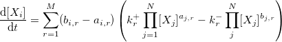
we used [] to represent the concentration.

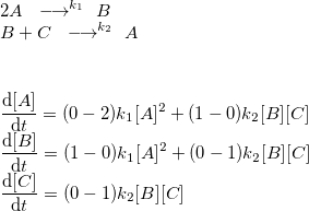
This may look scary, so here is an example with one-way reactions (like the ones for argon):

Exercises

Exercise 1

• What is the unit of the time derivative of the concentration (source term)? What must be the unit of the rate constant for a reaction involving two reactants and what for a reaction involving three reactants?

Exercise 2 If the argon gas was without excited and ionized species, the concentration of argon could be calculated from the equation of state for ideal gas.

• Calculate the actual concentration of ground state argon in plasma given the gas temperature, gas pressure, and the concentration of excited and ionized species (Ar⁺, Ar^*, Ar⁺₂)

Exercise 3 Look at the reaction table picture, reactions 1, 3, 4.

• What is the unit of the constant in the exponential? What is its physical meaning?
• Which reaction do you think will be the most important ionization channel?

Exercise 4

• Using the reaction table picture express the time derivatives of concentration (source terms) of species: e, Ar⁺, Ar^*, Ar⁺₂.

Exercise 5

• Complete the script. In particular, you need to:
  1. Write the expressions for the source terms (SArs,SArp,SAr2p and Se).
  2. Create the functions for rate constants f_k[1-11](Te,Tg)
  3. Run the script and decide if the output makes sense.

Exercise 6 Try increasing and decreasing the electron temperature and answer the following questions:

• How does the equilibrium electron density change and why?
• How does the ignition time change?
• What is the dominant ion in the ignition phase and what is the dominant ion when the plasma stabilizes? Does the dominance of the two ions change with electron temperature?

Exercise 7 Run the program for your chosen value of electron temperature and for pressures of 10³, 10⁴, 10⁵ and 10⁶ Pa and answer the following questions:

• How does the equilibrium electron density change and why?
• How does the ignition time change?

Advanced Exercise

• Modify the program in the previous section so that it solves the system of equations for several values of T_e/p and plots the steady-state number densities as functions of T_e/p. You can do this by adding a for loop. What makes this exercise difficult is the fact that the ignition time changes quite quickly with electron temperature and pressure. Therefore, the time interval has to be updated in each iteration according to the current value of T_e and p, otherwise the solution will take very long.

Implementation

The details of the script are discussed below.

import numpy as np
from scipy.integrate import odeint
import matplotlib.pyplot as plt 
p = 1e5
kB = 1.38e-23
Tg = 400.0
Te = 2.0

We import NumPy, the ODE solver and a plotting package. Then we define some constants.

tsteps = 1000
tspan = np.logspace(-11,-6,tsteps)

nArs_init = 1e12 # excited species
nArp_init = 1e12 # positive atoms
nAr2p_init = 1e12 # positive molecule
ne_init = nArp_init +  nAr2p_init # electron density
initial = [nArs_init, nArp_init, nAr2p_init, ne_init]

To solve the system of ODEs, we need to define the time span of the integration and the initial conditions.

def odefun(y,t):
    nArs = y[0]
    nArp = y[1]
    nAr2p = y[2]
    ne = y[3]

    nAr = p/(kB*Tg) - nArs - 0.5*nAr2p - nArp
    k1 = f_k1(Te,Tg)    
    k2 = f_k2(Te,Tg)
    k3 = f_k3(Te,Tg)
    k4 = f_k4(Te,Tg)
    k5 = f_k5(Te,Tg)
    k6 = f_k6(Te,Tg)
    k7 = f_k7(Te,Tg)
    k8 = f_k8(Te,Tg)
    k9 = f_k9(Te,Tg)
    k10 = f_k10(Te,Tg)
    k11 = f_k11(Te,Tg)

    SArs = k1*ne*nAr\
            -k2*ne*nArs\
            -k4*ne*nArs\
            +k6*ne*nAr2p\
            -2*k10*nArs**2\
            -k11*nArs*nAr
    #You need to fill in the correct expressions
    SArp = 1.0
    SAr2p = 1.0
    Se = 1.0

    return np.array([SArs,SArp,SAr2p,Se])

This is the first derivatives function. The functions for the rate constants are missing, you will need to implement them, as well as the right-hand sides for the derivatives.

y = odeint(odefun,initial,tspan) 

We use the odeint() function to solve the problem numerically.

nAr = p/(kB*Tg) - y[:,0]- 0.5*y[:,2]- y[:,1]

plt.loglog(tspan,nAr,'c',basex=10, label='Ar')
plt.loglog(tspan,y[:,0],'r',basex=10, label='Ar^*')
plt.loglog(tspan,y[:,1],'b',basex=10, label='Ar^+')
plt.loglog(tspan,y[:,2],'m',basex=10, label='Ar_2^+')
plt.loglog(tspan,y[:,3],'k',basex=10, label='el.')
plt.show()

Finally, we plot our results using log-log plots.