Home
SalsaTS is an web application developed for analyzing the observational data from the SALSA Onsala radio telescope. This document will describe how to use the tool. To use it, please visit https://appolloford.github.io/salsa-ts/.
SALSA is a collection of a few small (2.3m) radio telescopes situated at Onsala Space Observatory in Sweden. The telescopes are open to everyone to do observations. As many other observational data, the telescopes export the data in FITS format. A popular way to read these files is utilizing the Astropy package. However, this may not be friendly for the users without programming experience. Therefore, it is important to have a graphic user interface to help users read and analyze the observational results.
There was two tools developed before:
- Salsa-J: a software package that is used to reduce spectral data from the SALSA telescopes, but can also be used as a simple image editor and processor. A spectral module with functionality to reduce SALSA data is available. The main advantage of SalsaJ is its easy- to-use point-and-click interface. The main disadvantage is that reducing many spectra can be tedious. SalsaJ can be downloaded at the SALSA website. SalsaJ was developed for the European Hands-On Universe (EU-HOU) project, an education project aimed to provide interesting exercises in the field of astronomy for high school students.
- SalsaSpectrum is a data reduction environment written in the popular mathematical soft- ware Matlab - aimed for reduction of data from SALSA Onsala, developed by Daniel Dahlin.
However, these tools rely on Java and MATLAB, and have trouble to distribute. SalsaTS is then developed as a web application and deployed on Github pages to make sure users can access the website from anywhere.
In the next chapter, we will introduce the new graphic user interface.
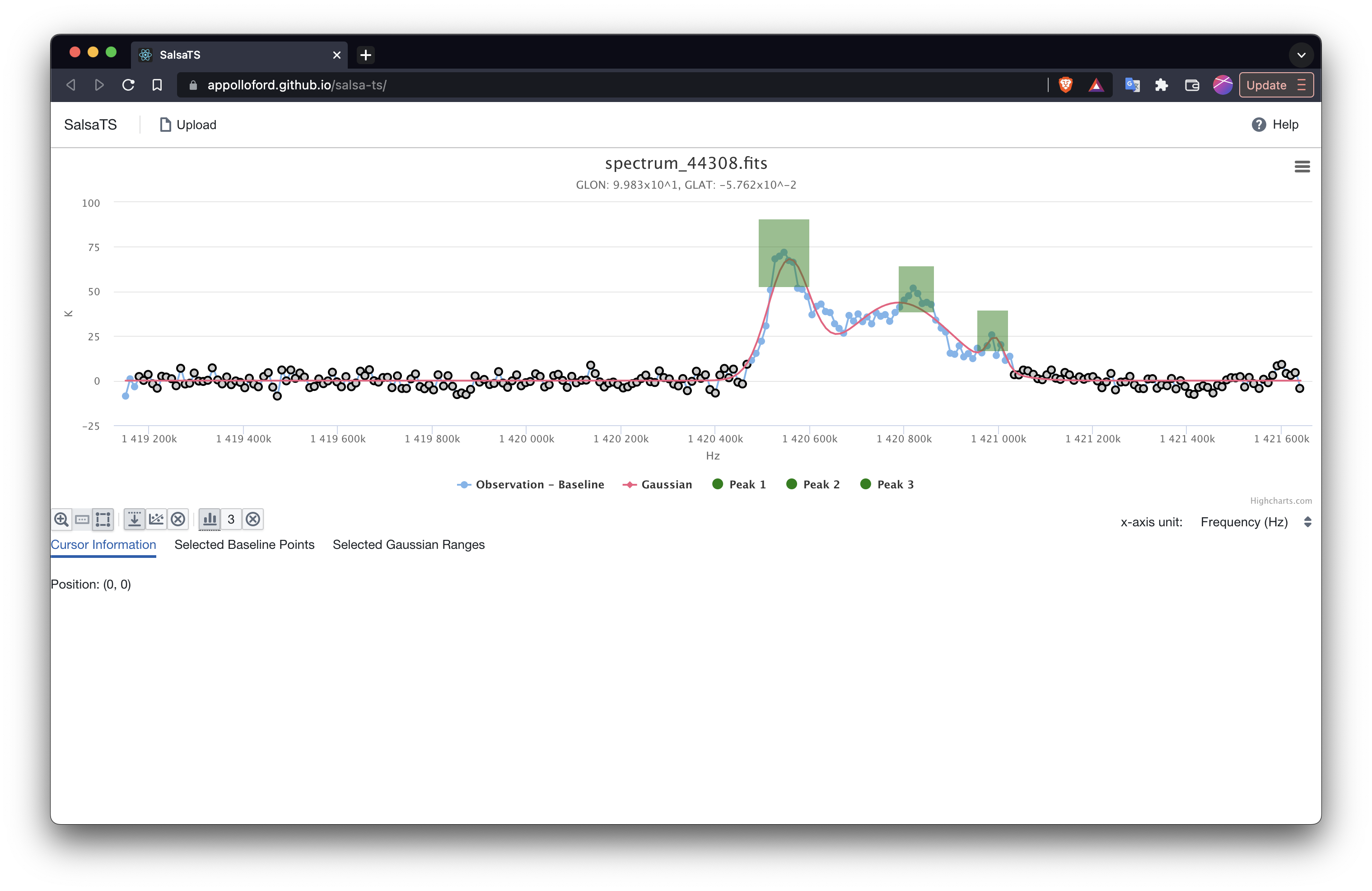
In this section, we will show the basic usage by reproducing the following image:
- To start, connect to the SalsaTS website. You will see the blank page:

- Upload a fits file from SALSA observations by clicking the
Uploadbutton on the top left. If you see the button is disabled, please wait for a few seconds. The website is loading some required tools. If you need a sample fits file, please check the tests folder of the repository.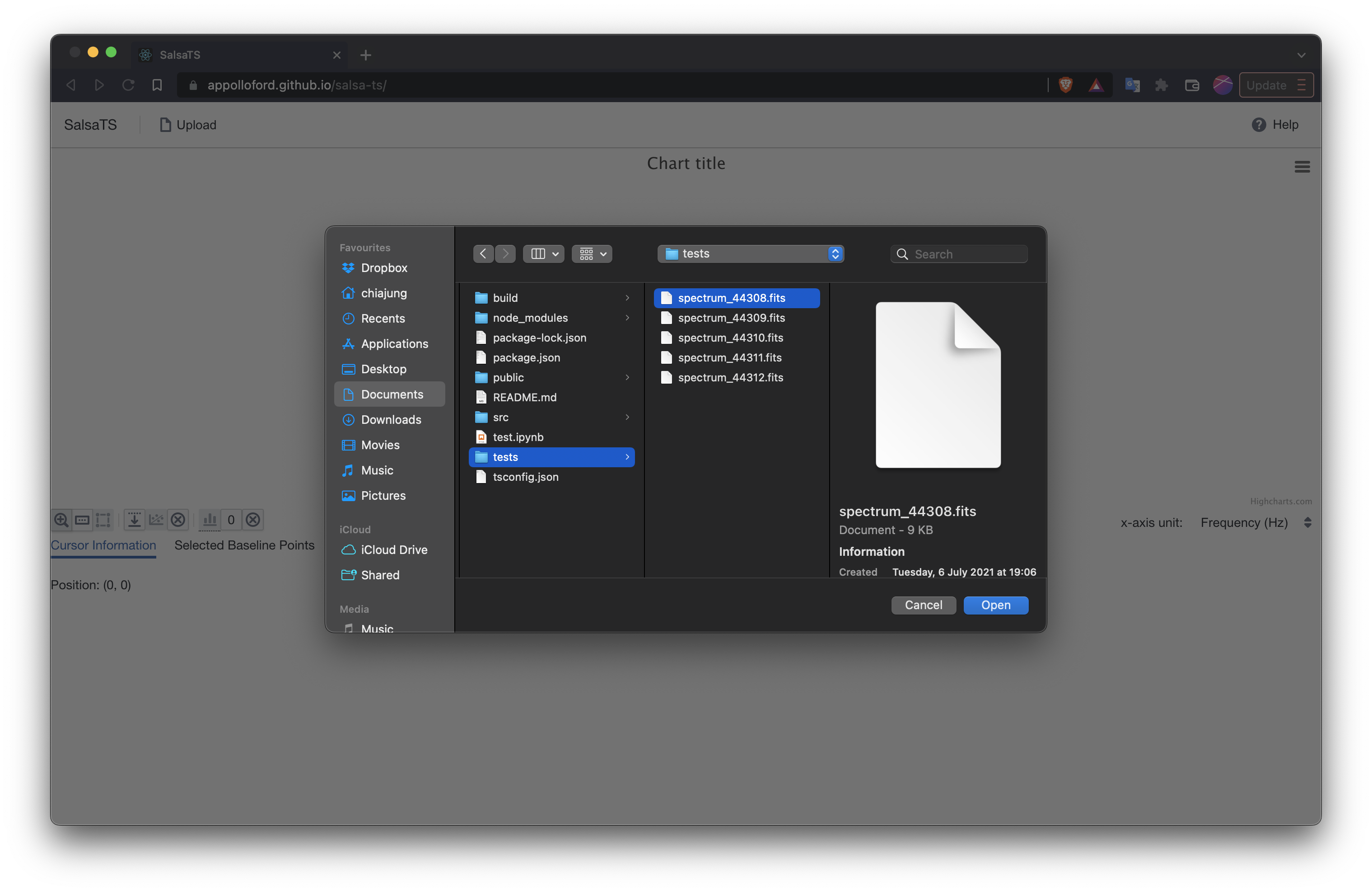
- You will see the spectrum displayed on the screen.

- Click the selecting button to start the selection of baseline points. The shadow shows the range chosen by cursor dragging.

- With the points selected, we can click the button to fit a baseline. The default is fitting to a second order polynomial.

- Click the button to subtract the baseline

- Click the drawing button to draw rectangles on the profile. The rectangles contraint the gaussian fitting, what we are doing in the next step. You can draw multiple rectangles on the profile. Each rectangle set the upper/lower limits of the peak and the FWHM of a gaussian.


- Click the button to turn on gaussian fitting. You can choose how many peaks you would like to fit. If the number of peaks is more than the number of rectangles, it will try to find the additional peaks in the global range. If the number of peaks is less than the number of rectangles, it will try to match the rectangles in the order of drawing.


- Now, you get the result we have shown in the beginning.

-
File Uploader: Upload files to the application. Although the application is opened in browser, the backend is executed locally. The file will not be uploaded to any server. Currently, you can only open one file at a time.
-
Help: External link to this page.
-
Spectrum Renderer: Display the spectrum profile. The title shows the filename and the subtitle shows the coordinates. The menu has the options of file saving (Highcharts built-in functions).
-
Cursor Actions: Set the action done by dragging cursor on the profile. Currently there are three modes: zoom, selecting baseline points, and drawing rectangles for constrainting gaussian fitting. Default is zoom.
-
Baseline Options (from left to right):
- baseline subtraction: display the spectrum that has subtracted the baseline
- baseline fitting: fit baseline (only once). If more points are added, users have to click the button to update the baseline result.
- clean: clean the selected baseline points and baseline
-
Gaussian Options (from left to right):
- gaussian fitting: fit gaussian. If the button is pressed, it will keep the result updated when more constraints/peaks are added.
- number of peaks: set the number of peaks users would like to fit to the spectrum. Default is 0.
- clean: clean all the constraints and the fitted gaussians.
-
X-axis unit: set the x-axis unit of the spectrum.
-
Cursor Information Tab: show the cursor position.
-
Baseline Information Tab: show the table of the points selected for baseline fitting
-
Gaussian Information Tab: show the table of the rectangles drawn on the profile.
TBD
If you find something that seems strange or doesn't work, please tell us.
You can report problems in two ways: (1) Feel free to open an issue on github (2) You can also choose to send a mail to Chia-Jung Hsu ([email protected]).