-
Notifications
You must be signed in to change notification settings - Fork 19
First Argo Simulation Model
This basic example will help us cover the step-by-step process of creating a simple cost and profit model utilizing Argo's interface and compare it with a very simplistic model that does not use simulation. We will also discuss how to interpret results of the Argo model and perform risk assessment. The model is explained in-depth throughout this page, but you can follow along yourself using the basic simulation example model provided in Basic Simulation Model - Business Operating Cost Model.

The business operating cost example is modeled on a mobile food truck business. The goal is to calculate monthly Gross Profit, which is the difference between Revenue and Total Operating Cost. Total operating cost is defined as the sum of Fixed Costs and Variable Costs. Revenue is defined as the product of the number of units sold and price per unit.
The monthly operating cost for this business includes:
- Fixed Costs (e.g. Labor, Car Payments)
- Variable Costs (e.g. Gasoline, Cost of Units Sold)
Table of Contents
- Introduction
- Identifying Uncertainty Associated with Model Inputs
- Building a Simple Model
- Building a Simulation Model with Argo
- Model Analysis
The user-friendly Argo interface makes building a new simulation model very straightforward. You start by identifying all the variables necessary to calculate the final results. From these, you identify which variables are uncertain, and use the appropriate distribution function to calculate their uncertainty. Your final results will reflect these distributions and will allow you to use Argo to perform analysis.
Every model that involves risk assessment contains two types of variables: pre-determined variables and uncertain variables:
- Pre-determined variables refer to fixed values or functions of fixed values. Monthly car payments, employee's yearly salary (the sum of 12 monthly salaries), or a factory rent payment are examples of pre-determined variables.
- Uncertain variables are those variables that vary depending on internal or external factors. For instance, the price of gas on a given day, lending rates or quantity of a good demanded are all uncertain variables. Uncertain variables either takes on values according to well-known probability distributions or are functions of probability distributions and pre-determined variables. For instance, the price of gasoline could be modeled using a Triangular distribution with parameters of minimum price, most likely price and maximum price. Other uncertain variables are outputs of combinations of several distributions and/or pre-determined variables. For example, monthly cost of gasoline determined by the price of gasoline (modeled via a Triangular distribution) multiplied by a pre-determined number of gallons purchased.
Some inputs to the business operating cost model are subject to variation. For example, gas prices are likely to vary each time the mobile food truck is refueled. This variation in gas price will result in uncertainty in total operating cost which in turn will contribute to the uncertainty in model outputs such as net profit. The gas price example illustrates the importance of identifying and including uncertainty associated with model inputs for effective analysis of model outputs. Considering the business operating cost scenario, you identify and quantify the following sources of uncertainty:
Monthly Variable Costs
- Uncertain Input: Gasoline - Based on current gasoline prices, you expect to $200 to be the most likely monthly cost of gasoline. Taking into account changing gas prices, you estimate the minimum and maximum monthly cost of gasoline to be $175 and $250 respectively.
- Uncertain Input: Cost per Unit - You find that unit costs will change minimally based on swaying food prices. You expect the most likely cost per sandwich will be $4.00, the minimum cost per sandwich will be $3.75, and the maximum cost per sandwich will be $4.25.
Sales Forecast
Sandwich sales will change based on consumer demand and competition against other food trucks in the area. You have an idea of the three possible scenarios: Optimistic (best case), Moderate (most likely), and Pessimistic (worst case).
- Uncertain Input: Price per Unit - Sandwiches are currently priced at $10 per sandwich (optimistic case). In the moderate case sandwiches would be priced at $9 a sandwich and in the worst case, $8 a sandwich.
- Uncertain Input: Number of Units Sold - In the optimistic case, you expect to sell 1000 sandwiches. In the moderate case you expect to sell 750 sandwiches. In the pessimistic case you expect to sell only 500 sandwiches.
For ease of interpretation, in the Argo model the above uncertain inputs are each modeled using the triangular distribution.
First, we examine a simplistic model that computes averages of uncertain variables. The model shown below is located in the spreadsheet titled “Averages (Incorrect)” and calculates Gross Profit based on revenue and total costs.
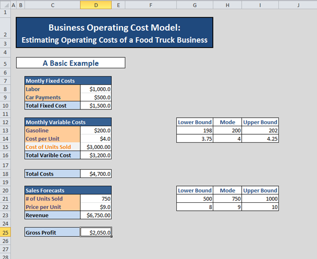
Note that all uncertain variables are calculated using averages of their corresponding lower bound, mode and upper bound values. This results in a weak analysis and misleading output that does not reflect any concept of risk or changing scenarios. We will now show how Argo can be used to solve this problem.
Now we discuss how to build a basic simulation model using Argo. The model shown below is located on the spreadsheet “Argo”. The goal of the model is to simulate how a desired result, in our case the Gross Profit, will vary as uncertain inputs within the model vary according to prescribed probability distributions.
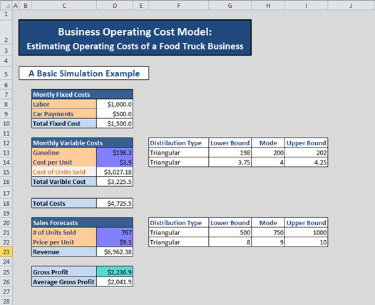
To create a dynamic and more accurate model, we will use Argo to simulate our uncertain variables and create distributions that reflect the probable outcomes of the variables.
As mentioned in section Identifying Uncertainty Associated with Model Inputs we will use triangular distribution to model all of our uncertain input variables. Triangular distribution is determined by three parameters: lower bound, mode, and upper bound. Note that distribution type and parameters for each of the uncertain variables are contained in the table to the right of the main input table.
Now, we will create a triangular distribution to determine gasoline cost. First, select cell D13 (the cell where distribution will be assigned). Then go to the Argo tab in the Excel ribbon and select Distribution ? Continuous ? Triangular as shown below.
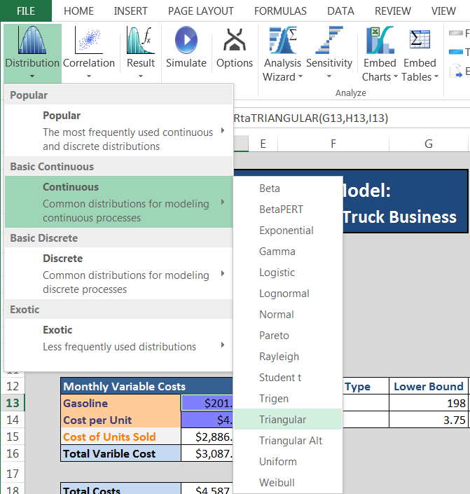
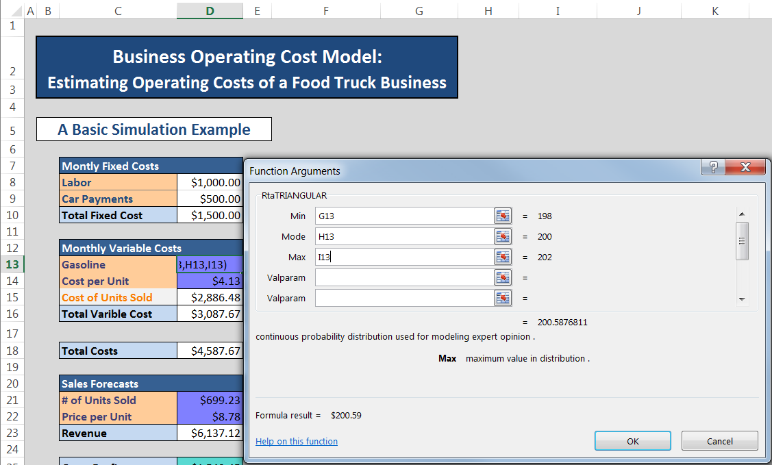
Once you click on the Triangular icon, a function form for a Triangular distribution pops up with options to enter parameters: Min, Mode, and Max (See figure below). Note that the name for the Triangular distribution in Argo is rtaTriangular (as shown in the top left hand corner of the function form). Link cells G13, I13, and H13 for Min, Mode and Max respectively and click OK. Now cell D13 contains formula =rtaTriangular(G13,H13,I13) and is shaded blue. A distribution could also be added to a cell manually by typing the distribution formula directly into the cell.
Repeat the process for Cost per Unit, # of Units Sold and Price per Unit (or copy paste the formula from cell D13). Now your model should look similar to the figure below. Values of probability distributions in your model will be different from the one below since these values are random samples of the distributions you defined.
We have now defined all of the uncertain variables in our model in terms of probability distributions.
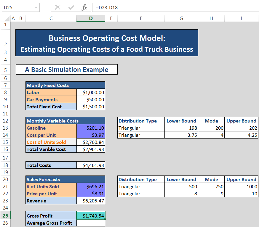
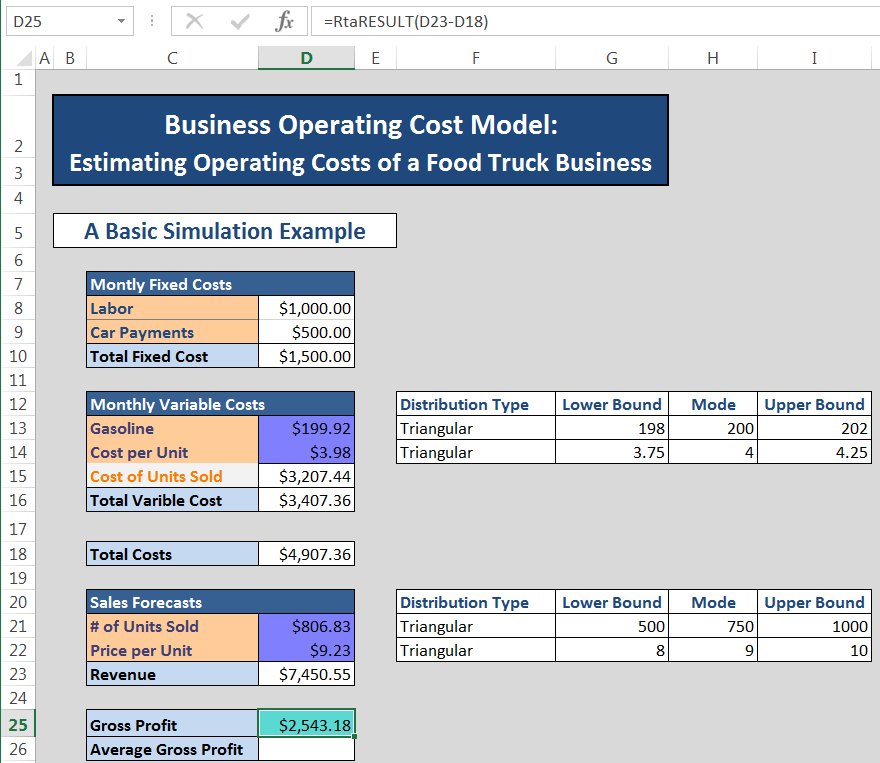
We've defined all uncertain variables that are described by probability distributions as described above, but the quantity we are really interested in is Gross Profit. Gross Profit is defined as Revenue minus Total Costs, so that formula in cell D25 is = D23-D18. To perform risk analysis on Gross Profit, we need to add its formula into the simulation, so that we keep track of how Gross Profit changes as all the distributions it depends on vary. We achieve this by designating cell D25 as a Result via Argo functions. To do so we select cell D25. Then, under the Argo tab in the Excel ribbon we select Result ? Add Result as shown below.
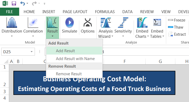
Notice that cell D25 now contains formula =rtaResult(D23-D18) as shown below. Notice RtaRESULT
function was applied to the entire original formula. A result could also be added into the model manually by typing the =rtaResult( … ) directly into the appropriate cell, where … stands for the original formula that is to be marked as a Result in the model. Since our model is basic, we do not have any more variables that need to be marked as Results in Argo. If you need to add more Results to your model, please repeat the steps described above.
Now we have defined all of uncertain variables in our model and we are ready to perform the simulation. During the simulation, Argo generates many (usually thousands) random samples of each distribution and stores these values in corresponding arrays. Moreover, Argo computes and stores arrays of values for all values marked as rtaResults. For all of the arrays that are collected, Argo computes and stores various statistical parameters of the data which allows to perform extensive risk analysis of the model.
To run the simulation, go to the Argo tab in the Excel ribbon and select Simulate.
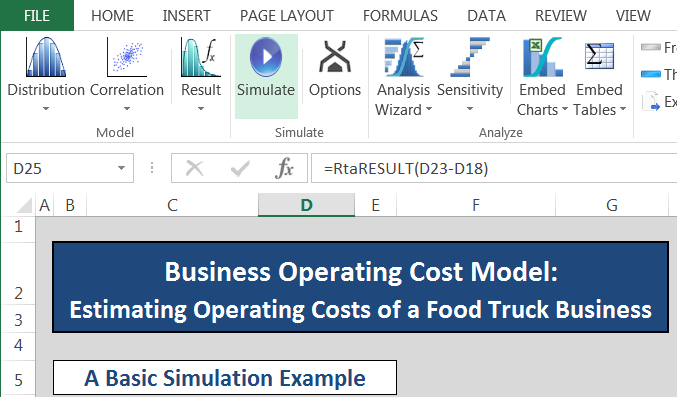
When the simulation is finished, the model will reflect updated values.
Now that we have created simulation of our model, we can perform statistical analysis. We do so by analyzing statistical parameters that Argo produced during the simulation. We discuss three ways of performing analysis in this section:
- Argo's OP functions which allow manual access to data produced by Argo and its statistical parameters via Excel formulas.
- Argo's Analysis Wizard feature which provides a visual and quantitative representation of the data produced by Argo in an interactive review window.
- Argo's Embedded Charts feature which allows Excel charts to be embedded directly into worksheets.
As we mentioned in Model Analysis, Argo's OP functions allow the user to access the data produced by Argo during the simulation and its statistical parameters. The most basic function, Op, pulls the values from a simulation. Using the format =Op(), you can access as many values as you have simulated. We call each sampling of a distribution a trial. In our simulation we have produced 1000 trials for each distribution and thus for each result as well. Note that 1000 trials per simulation is the default value. It can be changed by going to Argo ? Options ? Simulation Preferences.
To access some values that were produced by Gross Profit in Cell D25, we will select some cells (10 in this example) and type in =Op(D25). Because we are looking at an array, rather than just pressing enter, we will press Ctrl-Shift-Enter, and voila:
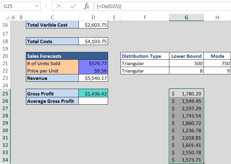
The figure above shows the first 10 values out of 1000 trials that were calculated for Gross Profit. Your numbers will not be the exact same as the ones shown here because each simulation is different, but they will all be within the parameters you defined based on the all the variables in the model.
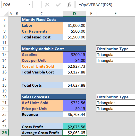
Most of the time we are interested in statistical parameters of the data that Argo produces. These parameters could also be accessed via OP functions. Most of the time we would like to see the average value of the data. We access it by writing =OpAVERAGE(D25) into the cell as shown below.
You can find all of the Argo OP functions by typing =op into a blank cell and using Excel's formula IntelliSense feature.

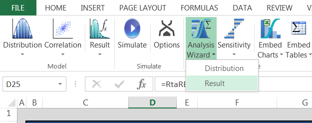
The Analysis Wizard allows for inspection of the uncertain distributions and results for the simulation runs.
For example, to get to the results on Gross Profit, click on Analysis Wizard Results and in the resulting pop-up check either D25 or Argo (to select all of the results).
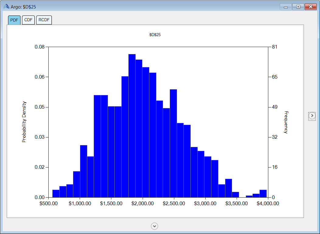
The tabs on the Analysis Wizard allow you to view the following plots: Probability Density Function, Cumulative Distribution Function, and a Reverse Cumulative Distribution Function.
The Analysis Wizard can also give us a numerical summary of the statistics of the distribution. On the right side of the wizard, you will find a single button (arrow embedded in a circle) that expands the right side of the chart.
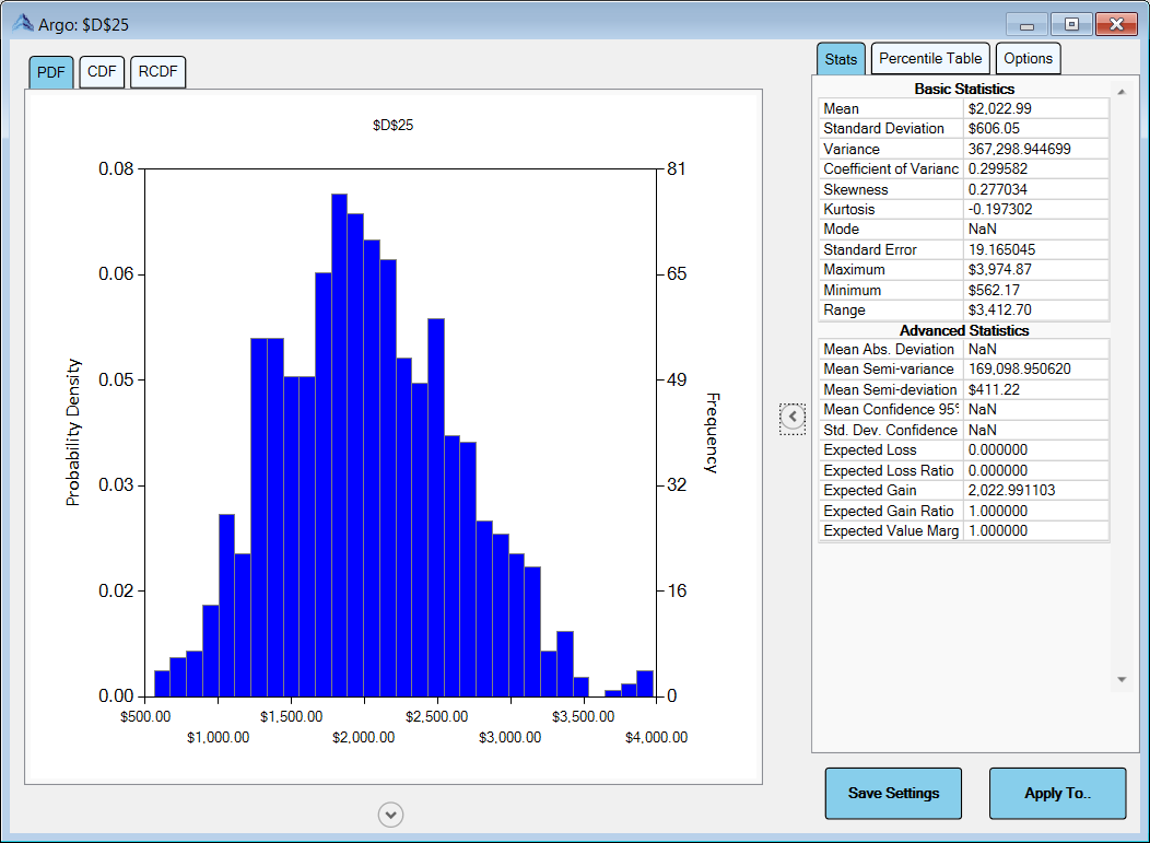
The side panel contains three tabs with detailed options:
-
Stats - the first tab provides basic and advanced statistics (e.g. mean, standard deviation, variance, skewness, range, etc.) on the variable, in this case the result in
D25 - Percentile Table - the second tab provides a table of percentiles and the option to select a percentile (e.g. 80th percentile) and have a marker appear on the distribution plot
- Options - the third tab provides access to options for customizing the plots
The Sensitivity Analysis allows us to view the factors influencing our selected variable. To look at the sensitivity of the Gross Profit, D25, relative to the uncertain inputs, select Sensitivity ? Correlation from the Argo ribbon. Select the Results checkbox and then click on the Analysis Wizard button at the bottom right to generate the sensitivity graph. There are a few options that can be set including the method (Pearson, Spearman), sort order, and graph display options.
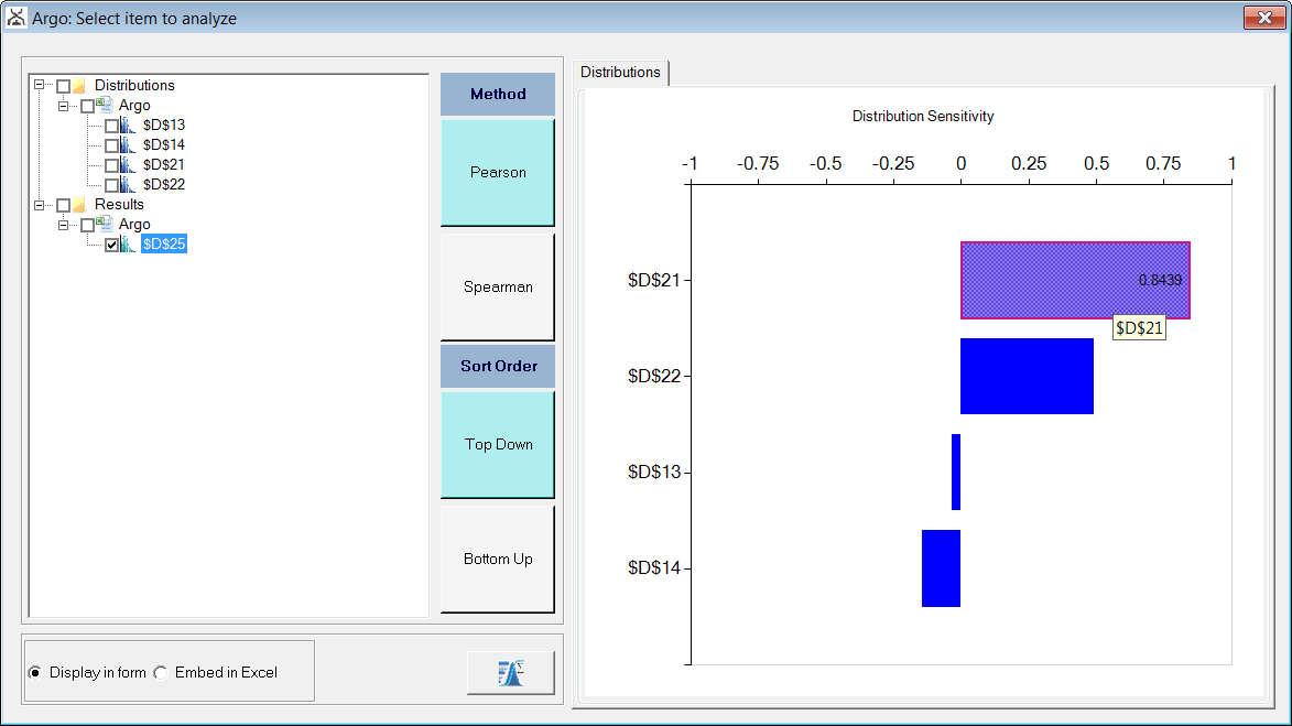
By hovering over the bars you can see the correlation with each variable. Here, we can see that the most correlated distribution to Gross Profit, with correlation coefficient .8439, is D21, # of units sold. Note: your correlation coefficients might be slightly different.
Another analysis option available in Argo is Embed Charts functionality. This option provides the ability to include the data that Argo produced in your workbook in the chart form. To access Embed Charts, click on Embed Charts button as shown below. Two options will come up: Distribution and Results.
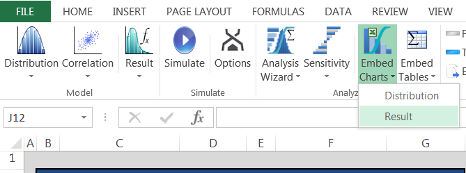
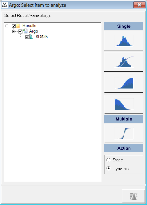
Embed Charts ? Results brings up the following dialog box which allows user to select options they'd like displayed (Frequency, CDF, RCDF and/or a combination chart). Select all four of the Single chart options and the Multiple chart option and then click the Analysis Wizard button in the bottom-right. Two new worksheets should be added to the workbook.
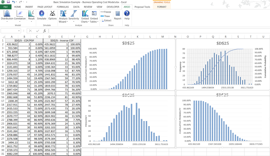
The first one, ChartSource-1, represents the single graphs and if all four options were selected will reflect those 4 charts and corresponding tables reflecting the frequency, CDF, and inverse CDF data used to generate the graphs. The second new worksheet, ChartSource-2, represents selecting the Multiple chart option.
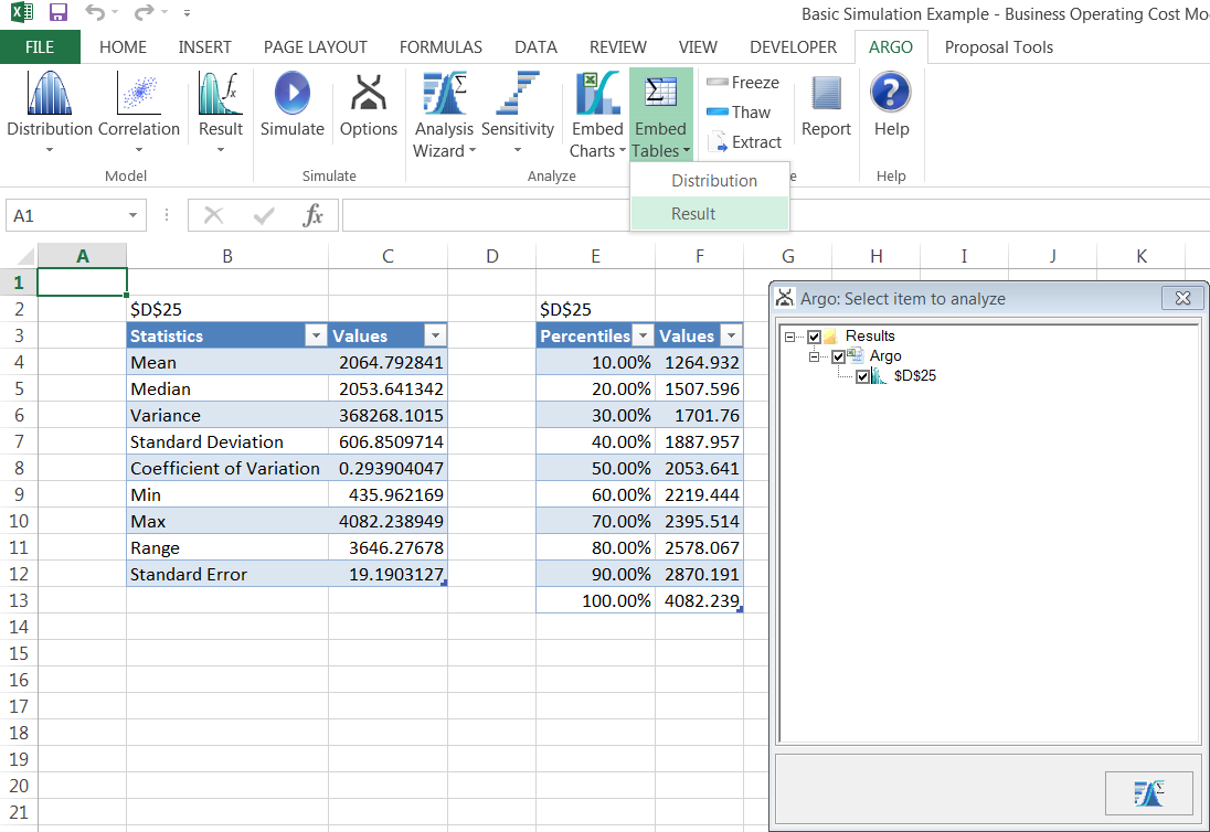
The last analysis option available in Argo is Embed Tables. Similar to Embed Charts, selecting the button provides two options, Distributions and Results. Selecting Results will open a dialog box and after choosing which results to display a new worksheet is added to the workbook. In this example the only result is D25 and the new worksheet, TableSource-1 shows summary statistics and percentile values for the Gross Profit, D25.
