Home
Welcome to MetaFX wiki page!
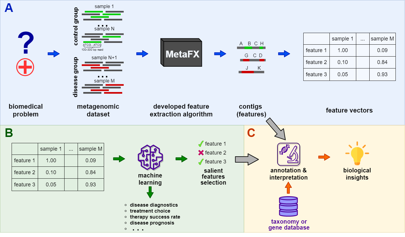
MetaFX (METAgenomic Feature eXtraction) is an open-source library for feature extraction from whole-genome metagenome sequencing data and classification of groups of samples.
The idea behind MetaFX is to introduce the feature extraction algorithm specific for metagenomics short reads data. It is capable of processing hundreds of samples 1-10 Gb each. The distinct property of suggest approach is the construction of meaningful features, which can not only be used to train classification model, but also can be further annotated and biologically interpreted.
To run MetaFX, one need to clone repo with all binaries.
git clone https://github.com/ctlab/metafx
cd metafx
Then add MetaFX binary directory to path.
export PATH=/path/to/metafx/bin:$PATHFor permanent use, add the above line to your ~/.profile or ~/.bashrc file.
Requirements:
- JRE 1.8 or higher
- python3
- python libraries listed in
requirements.txtfile. Can be installed using pip
python -m pip install --upgrade pip
pip install -r requirements.txt-
coreutils required for macOS (e.g.
brew install coreutils) - If you want to use
metafx metaspadespipeline, you will also need SPAdes software. Please follow their installation instructions (not recommended for first-time use). - If you want to use
metafx bandagepipeline, you will also need BandageNG software. Please follow installation instructions in wiki. Optionally, you may require SPAdes (see above).
Scripts have been tested under Ubuntu 18.04 LTS, Ubuntu 20.04 LTS, macOS 11 Big Sur, and macOS 12 Monterey, and should generally work on Linux/macOS.
To run MetaFX use the following syntax:
metafx <pipeline> [<Launch options>] [<Input parameters>]To view the list of supported pipelines run metafx -h or metafx --help.
To view help for launch options and input parameters for selected pipeline run metafx <pipeline> -h or metafx <pipeline> --help.
MetaFX supports both single-end and paired-end input files. For correct detection of paired-end reads, files should be named with suffixes "_R1"&"_R2" or "_r1"&"_r2" after sample name before extension. For example, sample_r1.fastq&sample_r2.fastq, or reads_R1.fq.gz&reads_R2.fq.gz.
By running MetaFX a working directory is created (by default ./workDir/).
All intermediate files and final results are saved there.
MetaFX is a toolbox with a lot of modules divided into three groups:
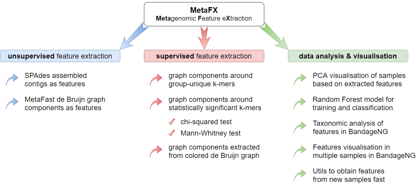
There are pipelines aimed to extract features from metagenomic dataset without any prior knowledge about samples and their relations. Algorithms perform (pseudo-)assembly of samples separately and construct the de Bruijn graph common for all samples. Further, graph components are extracted as features and feature table is constructed.
Performs unsupervised feature extraction and distance estimation via MetaFast (https://github.com/ctlab/metafast/).
metafx metafast -t 2 -m 4G -w wd_metafast -k 21 -i test_data/test*.fastq.gz -b1 100 -b2 500Input parameters
| parameter | description |
|---|---|
| -t, --threads <int> | number of threads to use [default: all] |
| -m, --memory <MEM> | memory to use (values with suffix: 1500M, 4G, etc.) [default: 90% of free RAM] |
| -w, --work-dir <dirname> | working directory [default: workDir/] |
| -k, --k <int> | k-mer size (in nucleotides, maximum value is 31) [mandatory] |
| -i, --reads <filenames> | list of reads files from single environment. FASTQ, FASTA, gzip- or bzip2-compressed [mandatory] |
| -b, --bad-frequency <int> | maximal frequency for a k-mer to be assumed erroneous [default: 1] |
| -l, --min-seq-len <int> | minimal sequence length to be added to a component (in nucleotides) [default: 100] |
| -b1, --min-comp-size <int> | minimum size of extracted components (features) in k-mers [default: 1000] |
| -b2, --max-comp-size <int> | maximum size of extracted components (features) in k-mers [default: 10000] |
| --kmers-dir <dirname> | directory with pre-computed k-mers for samples in binary format [optional] |
| --skip-graph | if TRUE skip de Bruijn graph and fasta construction from components [default: False] |
Output files
For backward compatibility with supervised feature extraction, every sample belongs to category all.
| file | description |
|---|---|
| wd_metafast/categories_samples.tsv | tab-separated file with 3 columns: <category>\t<present_samples>\t<absent_samples> |
| wd_metafast/samples_categories.tsv | tab-separated file with 2 columns: <sample_name>\t<category> |
| wd_metafast/feature_table.tsv | tab-separated numeric features file: rows – features, columns – samples |
| wd_metafast/contigs_all/components.seq.fasta | contigs in FASTA format as features (suitable for annotation and biological interpretation) |
| wd_metafast/contigs_all/components-graph.gfa | de Bruijn graph of features in GFA format (suitable for visualisation in Bandage) |
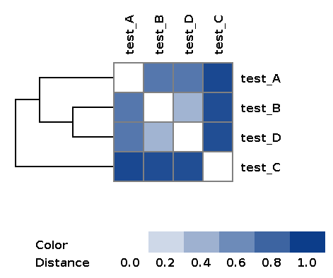
| wd_metafast/matrices/dist_matrix_<DATE_TIME>.txt | Distance matrix between every pair of samples built over feature table using Bray-Curtis dissimilarity |
| wd_metafast/matrices/dist_matrix_<DATE_TIME>_heatmap.png | Heatmap and dendrogram of samples based on distance matrix |
Example of the resulting heatmap with dendrogram:
Performs unsupervised feature extraction and distance estimation via metaSpades (https://github.com/ablab/spades)
NB: Requires SPAdes installation. Please follow their installation instructions
metafx metaspades -t 2 -m 4G -w wd_metaspades -k 21 -i test_data/test_*.fastq.gz -b1 500 -b2 5000Input parameters
| parameter | description |
|---|---|
| -t, --threads <int> | number of threads to use [default: all] |
| -m, --memory <MEM> | memory to use (values with suffix: 1500M, 4G, etc.) [default: 90% of free RAM] |
| -w, --work-dir <dirname> | working directory [default: workDir/] |
| -k, --k <int> | k-mer size (in nucleotides, maximum value is 31) [mandatory] |
| -i, --reads <filenames> | list of PAIRED-END reads files from single environment. FASTQ, FASTA, gzip-compressed [mandatory] |
| --separate | if TRUE use every spades contig as a separate feature (-l, -b1, -b2 ignored) [default: False] |
| -l, --min-seq-len <int> | minimal sequence length to be added to a component (in nucleotides) [default: 100] |
| -b1, --min-comp-size <int> | minimum size of extracted components (features) in k-mers [default: 1000] |
| -b2, --max-comp-size <int> | maximum size of extracted components (features) in k-mers [default: 10000] |
| --kmers-dir <dirname> | directory with pre-computed k-mers for samples in binary format [optional] |
| --skip-graph | if TRUE skip de Bruijn graph and fasta construction from components [default: False] |
Output files
For backward compatibility with supervised feature extraction, every sample belongs to category all.
| file | description |
|---|---|
| wd_metaspades/categories_samples.tsv | tab-separated file with 3 columns: <category>\t<present_samples>\t<absent_samples> |
| wd_metaspades/samples_categories.tsv | tab-separated file with 2 columns: <sample_name>\t<category> |
| wd_metaspades/feature_table.tsv | tab-separated numeric features file: rows – features, columns – samples |
| wd_metaspades/contigs_all/components.seq.fasta | contigs in FASTA format as features (suitable for annotation and biological interpretation) |
| wd_metaspades/contigs_all/components-graph.gfa | de Bruijn graph of features in GFA format (suitable for visualisation in Bandage) |
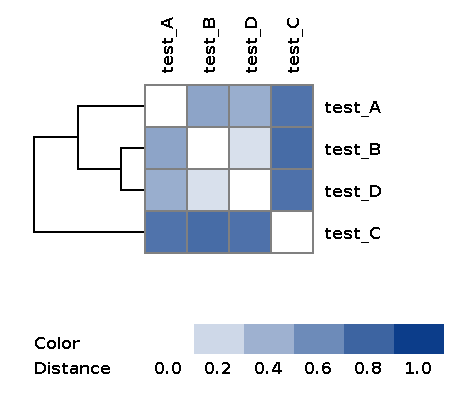
| wd_metaspades/matrices/dist_matrix_<DATE_TIME>*.txt | Distance matrix between every pair of samples built over feature table using Bray-Curtis dissimilarity |
| wd_metaspades/matrices/dist_matrix_<DATE_TIME>*_heatmap.png | Heatmap and dendrogram of samples based on distance matrix |
Example of the resulting heatmap with dendrogram:
There are pipelines aimed to extract group-relevant features based on metadata about samples such as diagnosis, treatment, biochemical results, etc. Dataset is split into groups of samples based on provided metadata information and group-specific features are constructed based on de Bruijn graphs. The resulting features are combined into feature table.
Performs supervised feature extraction using group-specific k-mers. K-mer is considered to be group-specific if it is present in at least G samples of certain group and absent in all other samples.
metafx unique -t 2 -m 4G -w wd_unique -k 21 -i test_data/sample_list_train.txtInput parameters
| parameter | description |
|---|---|
| -t, --threads <int> | number of threads to use [default: all] |
| -m, --memory <MEM> | memory to use (values with suffix: 1500M, 4G, etc.) [default: 90% of free RAM] |
| -w, --work-dir <dirname> | working directory [default: workDir/] |
| -k, --k <int> | k-mer size (in nucleotides, maximum value is 31) [mandatory] |
| -i, --reads <filename> | tab-separated file with 2 values in each row: <path_to_file>\t<category> [mandatory] |
| -b, --bad-frequency <int> | maximal frequency for a k-mer to be assumed erroneous [default: 1] |
| --min-samples <int> | k-mer is considered group-specific if present in at least G samples of that group. G iterates in range [--min-samples; --max-samples] [default: 2] |
| --max-samples <int> | k-mer is considered group-specific if present in at least G samples of that group. G iterates in range [--min-samples; --max-samples] [default: #{samples in category}/2 + 1] |
| --depth <int> | depth of de Bruijn graph traversal from pivot k-mers in number of branches [default: 1] |
| --kmers-dir <dirname> | directory with pre-computed k-mers for samples in binary format [optional] |
| --skip-graph | if TRUE skip de Bruijn graph and fasta construction from components [default: False] |
Output files
| file | description |
|---|---|
| wd_unique/categories_samples.tsv | tab-separated file with 3 columns: <category>\t<present_samples>\t<absent_samples> |
| wd_unique/samples_categories.tsv | tab-separated file with 2 columns: <sample_name>\t<category> |
| wd_unique/feature_table.tsv | tab-separated numeric features file: rows – features, columns – samples |
| wd_unique/contigs_<category>/components.seq.fasta | contigs in FASTA format as features (suitable for annotation and biological interpretation) |
| wd_unique/contigs_<category>/components-graph.gfa | de Bruijn graph of features in GFA format (suitable for visualisation in Bandage) |
Performs supervised feature extraction using chi-squared test for selection top significant k-mers. K-mer significance for a certain group is determined in two steps. Firstly, all k-mers are sorted based on p-value of chi-squared test. Secondly, top N k-mers are selected for each category (total N k-mers are selected in case of 2 or 3 categories).
metafx chisq -t 2 -m 4G -w wd_chisq -k 21 -i test_data/sample_list.txt -n 1000Input parameters
| parameter | description |
|---|---|
| -t, --threads <int> | number of threads to use [default: all] |
| -m, --memory <MEM> | memory to use (values with suffix: 1500M, 4G, etc.) [default: 90% of free RAM] |
| -w, --work-dir <dirname> | working directory [default: workDir/] |
| -k, --k <int> | k-mer size (in nucleotides, maximum value is 31) [mandatory] |
| -i, --reads <filename> | tab-separated file with 2 values in each row: <path_to_file>\t<category> [mandatory] |
| -n, --num-kmers <int> | number of most specific k-mers to be extracted [mandatory] |
| -b, --bad-frequency <int> | maximal frequency for a k-mer to be assumed erroneous [default: 1] |
| --depth <int> | depth of de Bruijn graph traversal from pivot k-mers in number of branches [default: 1] |
| --kmers-dir <dirname> | directory with pre-computed k-mers for samples in binary format [optional] |
| --skip-graph | if TRUE skip de Bruijn graph and fasta construction from components [default: False] |
Output files
| file | description |
|---|---|
| wd_chisq/categories_samples.tsv | tab-separated file with 3 columns: <category>\t<present_samples>\t<absent_samples> |
| wd_chisq/samples_categories.tsv | tab-separated file with 2 columns: <sample_name>\t<category> |
| wd_chisq/feature_table.tsv | tab-separated numeric features file: rows – features, columns – samples |
| wd_chisq/contigs_<category>/components.seq.fasta | contigs in FASTA format as features (suitable for annotation and biological interpretation) |
| wd_chisq/contigs_<category>/components-graph.gfa | de Bruijn graph of features in GFA format (suitable for visualisation in Bandage) |
Performs supervised feature extraction using statistically significant k-mers. K-mer significance for a certain group is determined in two steps. Firstly, Pearson's chi-squared test for homogeneity filters out k-mers, which have the same distribution between categories. Secondly, for each pair of categories Mann–Whitney U test is applied to select k-mers with different occurrences between categories.
metafx stats -t 2 -m 4G -w wd_stats -k 21 -i test_data/sample_list.txt --pchi2 0.05 --pmw 0.05Input parameters
| parameter | description |
|---|---|
| -t, --threads <int> | number of threads to use [default: all] |
| -m, --memory <MEM> | memory to use (values with suffix: 1500M, 4G, etc.) [default: 90% of free RAM] |
| -w, --work-dir <dirname> | working directory [default: workDir/] |
| -k, --k <int> | k-mer size (in nucleotides, maximum value is 31) [mandatory] |
| -i, --reads <filename> | tab-separated file with 2 values in each row: <path_to_file>\t<category> [mandatory] |
| -b, --bad-frequency <int> | maximal frequency for a k-mer to be assumed erroneous [default: 1] |
| --pchi2 <float> | p-value for chi-squared test [default: 0.05] |
| --pmw <float> | p-value for Mann–Whitney test [default: 0.05] |
| --depth <int> | depth of de Bruijn graph traversal from pivot k-mers in number of branches [default: 1] |
| --kmers-dir <dirname> | directory with pre-computed k-mers for samples in binary format [optional] |
| --skip-graph | if TRUE skip de Bruijn graph and fasta construction from components [default: False] |
Output files
| file | description |
|---|---|
| wd_stats/categories_samples.tsv | tab-separated file with 3 columns: <category>\t<present_samples>\t<absent_samples> |
| wd_stats/samples_categories.tsv | tab-separated file with 2 columns: <sample_name>\t<category> |
| wd_stats/feature_table.tsv | tab-separated numeric features file: rows – features, columns – samples |
| wd_stats/contigs_<category>/components.seq.fasta | contigs in FASTA format as features (suitable for annotation and biological interpretation) |
| wd_stats/contigs_<category>/components-graph.gfa | de Bruijn graph of features in GFA format (suitable for visualisation in Bandage) |
Performs supervised feature extraction using group-colored de Bruijn graph. All k-mers are colored based on their relative occurrences in categories and further de Bruijn graph is split into colored components.
Important! This module supports up to 3 categories of samples. If you have more, consider using other MetaFX modules.
metafx colored -t 2 -m 4G -w wd_colored -k 21 -i test_data/sample_list_3.txt --linear --n-comps 100 --perc 0.8Input parameters
| parameter | description |
|---|---|
| -t, --threads <int> | number of threads to use [default: all] |
| -m, --memory <MEM> | memory to use (values with suffix: 1500M, 4G, etc.) [default: 90% of free RAM] |
| -w, --work-dir <dirname> | working directory [default: workDir/] |
| -k, --k <int> | k-mer size (in nucleotides, maximum value is 31) [mandatory] |
| -i, --reads <filename> | tab-separated file with 2 values in each row: <path_to_file>\t<category> [mandatory] |
| -b, --bad-frequency <int> | maximal frequency for a k-mer to be assumed erroneous [default: 1] |
| --total-coverage | if TRUE count k-mers occurrences in colored graph as total coverage in samples, otherwise as number of samples [default: False] |
| --separate | if TRUE use only color-specific k-mers in components (does not work in --linear mode) [default: False] |
| --linear | if TRUE extract only linear components choosing the best path on each graph fork [default: False] |
| --n-comps <int> | select not more than <int> components for each category [default: -1, means all components] |
| --perc <float> | relative abundance of k-mer in category to be considered color-specific [default: 0.9] |
| --kmers-dir <dirname> | directory with pre-computed k-mers for samples in binary format [optional] |
| --skip-graph | if TRUE skip de Bruijn graph and fasta construction from components [default: False] |
Output files
| file | description |
|---|---|
| wd_colored/categories_samples.tsv | tab-separated file with 3 columns: <category>\t<present_samples>\t<absent_samples> |
| wd_colored/samples_categories.tsv | tab-separated file with 2 columns: <sample_name>\t<category> |
| wd_colored/feature_table.tsv | tab-separated numeric features file: rows – features, columns – samples |
| wd_colored/contigs_<category>/components.seq.fasta | contigs in FASTA format as features (suitable for annotation and biological interpretation) |
| wd_colored/contigs_<category>/components-graph.gfa | de Bruijn graph of features in GFA format (suitable for visualisation in Bandage) |
There are pipelines for analysis of the feature extraction results. Methods for samples similarity visualisation and training machine learning models are implemented. Classification models can be trained to predict samples' properties based on extracted features and to efficiently process new samples from the same environment.
Results of one of feature extraction MetaFX modules are required for further analysis
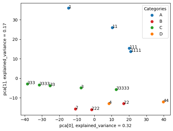
Performs PCA dimensionality reduction and visualisation of samples based on extracted features.
metafx pca -w wd_pca -f wd_stats/feature_table.tsv -i wd_stats/samples_categories.tsv --showInput parameters
| parameter | description |
|---|---|
| -w, --work-dir <dirname> | working directory [default: workDir/] |
| -f, --feature-table <filename> | file with feature table in tsv format: rows – features, columns – samples ("workDir/feature_table.tsv" can be used) [mandatory] |
| -i, --metadata-file <filename> | tab-separated file with 2 values in each row: <sample>\t<category> ("workDir/samples_categories.tsv" can be used) [optional, default: None] |
| --name <filename> | name of output image in workDir [optional, default: pca] |
| --show | if TRUE print samples' names on plot [optional, default: False] |
Output files
| file | description |
|---|---|
| wd_pca/pca.png | plot of 2-dimensional PCA in png format |
| wd_pca/pca.svg | plot of 2-dimensional PCA in svg format |
Example of the resulting PCA plot:
Executes Random Forest machine learning algorithm to train classification model based on extracted features.
metafx fit -w wd_fit -f wd_unique/feature_table.tsv -i wd_unique/samples_categories.tsvInput parameters
| parameter | description |
|---|---|
| -w, --work-dir <dirname> | working directory [default: workDir/] |
| -f, --feature-table <filename> | file with feature table in tsv format: rows – features, columns – samples ("workDir/feature_table.tsv" can be used) [mandatory] |
| -i, --metadata-file <filename> | tab-separated file with 2 values in each row: <sample>\t<category> ("workDir/samples_categories.tsv" can be used) [mandatory] |
| --name <filename> | name of output trained model in workDir [optional, default: rf_model] |
Output files
| file | description |
|---|---|
| wd_fit/rf_model.joblib | binary file with pre-trained classification model suitable for metafx predict module or further analysis |
This module processes new samples and counts feature values based on previously extracted features.
It can be used in the following case. A dataset with known samples categories have been processed, i.e. features were extracted and classification model was trained via fit or cv method.
Further new samples with unknown categories are needed to be studied.
Samples should be preprocessed with current calc_features method to get feature table, which can be used in predict module.
metafx calc_features -t 2 -m 4G -w wd_calc_features -k 21 -d wd_unique \
        -i test_data/test_A_R1.fastq.gz test_data/test_A_R2.fastq.gz \
           test_data/test_B_R1.fastq.gz test_data/test_B_R2.fastq.gz \
           test_data/test_C_R1.fastq.gz test_data/test_C_R2.fastq.gz
Input parameters
| parameter | description |
|---|---|
| -t, --threads <int> | number of threads to use [default: all] |
| -m, --memory <MEM> | memory to use (values with suffix: 1500M, 4G, etc.) [default: 90% of free RAM] |
| -w, --work-dir <dirname> | working directory [default: workDir/] |
| -k, --k <int> | k-mer size (in nucleotides, maximum value is 31) [mandatory] |
| -i, --reads <filenames> | list of reads files from single environment. FASTQ, FASTA, gzip- or bzip2-compressed [mandatory] |
| -d, --feature-dir <dirname> | directory containing folders with components.bin file for each category and categories_samples.tsv file. Usually, it is workDir/ from other MetaFX modules (unique, stats, colored, metafast, metaspades) [mandatory] |
| -b, --bad-frequency <int> | maximal frequency for a k-mer to be assumed erroneous [default: 1] |
| --kmers-dir <dirname> | directory with pre-computed k-mers for samples in binary format [optional] |
Output files
| file | description |
|---|---|
| wd_calc_features/feature_table.tsv | tab-separated numeric features file: rows – features, columns – samples |
Executes Random Forest machine learning method to classify new samples based on pre-trained model.
Generally, --feature-table is obtained via MetaFX calc_features module and --model via MetaFX fit or cv module.
metafx predict -w wd_predict -f wd_calc_features/feature_table.tsv --model wd_fit/rf_model.joblibInput parameters
| parameter | description |
|---|---|
| -w, --work-dir <dirname> | working directory [default: workDir/] |
| -f, --feature-table <filename> | file with feature table in tsv format: rows – features, columns – samples ("workDir/feature_table.tsv" can be used) [mandatory] |
| --model <filename> | file with pre-trained classification model, obtained via fit or cv module ("workDir/rf_model.joblib" can be used) [mandatory] |
| -i, --metadata-file <filename> | tab-separated file with 2 values in each row: <sample>\t<category> to check accuracy of predictions [optional, default: None] |
| --name <filename> | name of output file with samples predicted labels in workDir [optional, default: predictions] |
Output files
| file | description |
|---|---|
| wd_predict/predictions.tsv | tab-separated file with 2 values in each row: <sample name>\t<predicted category> |
Example of the resulting file:
$ cat wd_predict/predictions.tsv
test_A  A
test_C  C
test_B  B
As expected, all samples' categories were correctly predicted consistent with the file names.
Executes Random Forest machine learning algorithm to train classification model based on extracted features and check accuracy via cross-validation. Optionally, it can perform grid search of optimal parameters for classification model based on cross-validation.
metafx cv -t 2 -w wd_cv -f wd_stats/feature_table.tsv -i wd_stats/samples_categories.tsv -n 2 --gridInput parameters
| parameter | description |
|---|---|
| -t, --threads <int> | number of threads to use [default: 1] |
| -w, --work-dir <dirname> | working directory [default: workDir/] |
| -f, --feature-table <filename> | file with feature table in tsv format: rows – features, columns – samples ("workDir/feature_table.tsv" can be used) [mandatory] |
| -i, --metadata-file <filename> | tab-separated file with 2 values in each row: <sample>\t<category> ("workDir/samples_categories.tsv" can be used) [mandatory] |
| -n, --n-splits <int> | number of folds in cross-validation, must be at least 2 [optional, default: 5] |
| --name <filename> | name of output trained model in workDir [optional, default: rf_model_cv] |
| --grid | if TRUE, perform grid search of optimal parameters for classification model [optional, default: False] |
Output files
| file | description |
|---|---|
| wd_cv/rf_model_cv.joblib | binary file with pre-trained classification model suitable for metafx predict module or further analysis |
Executes Random Forest machine learning algorithm to train classification model based on extracted features and immediately apply it to classify new samples.
It can be used in case when all samples are available at the beginning of the study, but only a part of them is labeled. And the goal is to classify the rest samples.
In that case --feature-table contains all samples, but --metadata-file contains information only about part of samples.
To model such a situation, we will use wd_colored/feature_table.tsv with 12 samples.
Also, we need to create special test_labels.tsv file with only 6 samples labeled.
$ echo -e "1\tA\n11\tA\n2\tB\n22\tB\n3\tC\n33\tC" > test_labels.tsv
$ cat test_labels.tsv
1	A
11	A
2	B
22	B
3	C
33	C
metafx fit_predict -w wd_fit_predict -f wd_colored/feature_table.tsv -i test_labels.tsvInput parameters
| parameter | description |
|---|---|
| -w, --work-dir <dirname> | working directory [default: workDir/] |
| -f, --feature-table <filename> | file with feature table in tsv format: rows – features, columns – samples ("workDir/feature_table.tsv" can be used) [mandatory] |
| -i, --metadata-file <filename> | tab-separated file with 2 values in each row: <sample>\t<category> ("workDir/samples_categories.tsv" can be used) [mandatory] |
| --name <filename> | name of output trained model in workDir [optional, default: model] |
Output files
| file | description |
|---|---|
| wd_fit_predict/model.joblib | binary file with pre-trained classification model suitable for metafx predict module or further analysis |
| wd_fit_predict/model.tsv | tab-separated file with 2 values in each row: <sample name>\t<predicted category> |
Example of the resulting file:
$ cat wd_fit_predict/model.tsv
111 	A
1111	A
222 	B
333 	C
3333	C
33333	C
As expected, all samples' categories were correctly predicted (true labels can be found in wd_colored/samples_categories.tsv).
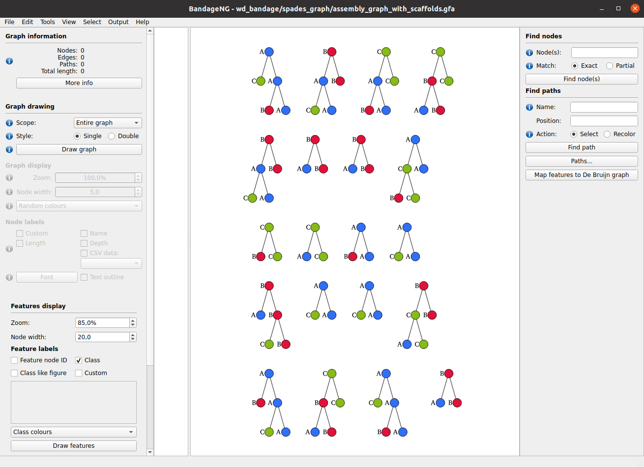
Performs preparation steps to visualise Machine Learning model and (optionally) the corresponding de Bruijn features graph in BandageNG. If model has not been trained, can itself train classification model.
Requires BandageNG installation. Here are instructions:
- Download the latest realised binary for your system (Linux or macOS): https://github.com/ctlab/BandageNG/releases
- Rename it to
BandageNGand make it executable (chmod u+x BandageNG) - Add the directory with
BandageNGto PATH (For permanent use, add this line to your ~/.profile or ~/.bashrc file)
export PATH=/path/to/BandageNG/:$PATHmetafx bandage -w wd_bandage -f wd_unique -n 20Input parameters
| parameter | description |
|---|---|
| -w, --work-dir <dirname> | working directory [default: workDir/] |
| -f, --feature-dir <dirname> | directory containing folders with contigs for each category, feature_table.tsv and categories_samples.tsv files. Usually, it is workDir from other MetaFX modules (unique, stats, colored, metafast, metaspades) [mandatory] |
| --model <filename> | file with pre-trained classification model, obtained via 'fit' or 'cv' module ("workDir/rf_model.joblib" can be used) [optional, if set '-n', '-d', '-e' will be ignored] |
| -n, --n-estimators <int> | number of estimators in classification model [optional] |
| -d, --max-depth <int> | maximum depth of decision tree base estimator [optional] |
| -e, --estimator [RF, ADA, GBDT] | classification model: RF – Random Forest, ADA – AdaBoost, GBDT – Gradient Boosted Decision Trees [optional, default: RF] |
| --draw-graph | if TRUE performs de Bruijn graph construction [default: False] |
| --gui | if TRUE opens Bandage GUI and draw images. Does NOT work on servers with command line interface only [default: False] |
| --name <filename> | name of output file with tree model in text format in workDir [optional, default: tree_model] |
Output files
| file | description |
|---|---|
| wd_bandage/tree_model.txt | pre-trained classification model in text format for visualisation in BandageNG |
| wd_bandage/tree_model.joblib | binary file with pre-trained classification model (created if new model was trained) |
| wd_bandage/spades_graph/assembly_graph_with_scaffolds.gfa | de Bruijn graph from features for BandageNG visualisation |
The resulting files can be visualised in BandageNG with the following steps:
- Open BandageNG program.
-
File → Load features forest: select
wd_bandage/tree_model.txtfile. - In the left panel in Features display section click Draw features button. Classification model of decision trees will be displayed.
-
File → Load graph: select
wd_bandage/spades_graph/assembly_graph_with_scaffolds.gfafile. - In the left panel in Graph drawing section click Draw graph button. De Bruijn graph constructed from features will be displayed.
- Features from classification model can be matched to graph. Select vertices in trees in the right part of the screen and then click Connect feature nodes with de bruijn nodes in the right panel.
In our example we obtain the following result (with only 3 first steps possible):
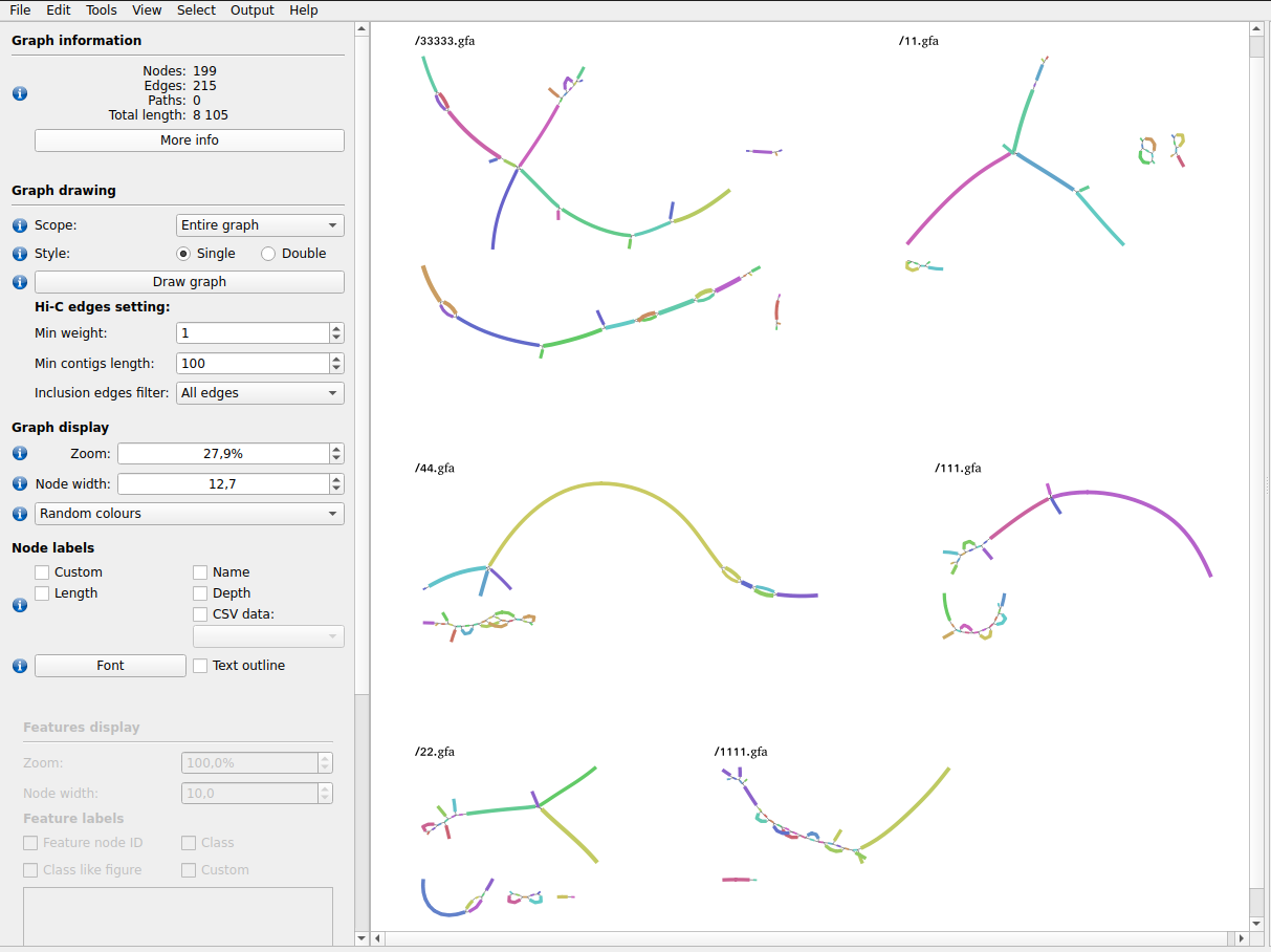
Selects samples containing the feature of interest with abundance above the threshold and build local de Bruijn graphs independently for each sample around the feature with MetaCherchant. Resulting graphs can be further analyzed in multi-graph mode in BandageNG.
We need to put all reads file into one directory for this module. For example, we can use soft links.
mkdir reads
ln -s `pwd`/test_data/3* reads/
ln -s `pwd`/test_data/4* reads/
ln -s `pwd`/test_data/test/* reads/
metafx feature_analysis -t 2 -m 4G -w wd_feat_analysis -k 21 -f wd_chisq/ -n A_15 -r reads/ --relab 0.5Input parameters
| parameter | description |
|---|---|
| -t, --threads <int> | number of threads to use [default: all] |
| -m, --memory <MEM> | memory to use (values with suffix: 1500M, 4G, etc.) [default: 90% of free RAM] |
| -w, --work-dir <dirname> | working directory [default: workDir/] |
| -k, --k <int> | k-mer size (in nucleotides, maximum value is 31) [mandatory] |
| -f, --feature-dir <dirname> | directory containing folders with contigs for each category, feature_table.tsv and categories_samples.tsv files. Usually, it is workDir from other MetaFX modules (unique, stats, colored, metafast, metaspades) [mandatory] |
| -n, --feature-name <string> | name of the feature of interest (should be one of the values from first column of feature_table.tsv) [mandatory] |
| -r, --reads-dir <dirname> | directory containing files with reads for samples. FASTQ, FASTA, gzip- or bzip2-compressed [mandatory] |
| --relab <int> | minimal relative abundance of feature in sample to include sample for further analysis [optional, default: 0.1] |
Output files
| file | description |
|---|---|
| wd_feat_analysis/samples_list_feature_<feature-name>.txt | list of selected samples containing feature above threshold |
| wd_feat_analysis/seq_feature_<feature-name>.fasta | nucleotide sequence for feature in FASTA format |
| wd_feat_analysis/graphs/ | directory with graphs for all selected samples |
All de Bruijn graphs saved to ${w}/graphs/ can be visualised simultaneously in BandageNG.
Such analysis requires BandageNG installation. Here are the instructions:
- Download the latest realised binary for your system (Linux or macOS): https://github.com/ctlab/BandageNG/releases
- Rename it to
BandageNGand make it executable (chmod u+x BandageNG) - Add the directory with
BandageNGto PATH (For permanent use, add this line to your ~/.profile or ~/.bashrc file)
export PATH=/path/to/BandageNG/:$PATHThe resulting files can be visualised in BandageNG with the following steps (detailed instructions):
- Open BandageNG program.
-
File → Load graphs from dir: select
wd_feat_analysis/graphs/directory. - In the left panel in Graph drawing section click Draw graph button. All de Bruijn graphs will be displayed.
In our example we obtain the following result:
There are modules to help to manipulate with data files and speed up MetaFX data processing.
This module processes reads files and extract k-mers for each sample separately.
It can reduce running time and RAM usage of other MetaFX modules, if the directory with extracted k-mers provided to other modules with --kmers-dir parameter.
metafx extract_kmers -t 2 -m 4G -w wd_extract_kmers -k 21 \
        -i test_data/test_A_R1.fastq.gz test_data/test_A_R2.fastq.gz \
           test_data/test_B_R1.fastq.gz test_data/test_B_R2.fastq.gz \
           test_data/test_C_R1.fastq.gz test_data/test_C_R2.fastq.gz
Input parameters
| parameter | description |
|---|---|
| -t, --threads <int> | number of threads to use [default: all] |
| -m, --memory <MEM> | memory to use (values with suffix: 1500M, 4G, etc.) [default: 90% of free RAM] |
| -w, --work-dir <dirname> | working directory [default: workDir/] |
| -k, --k <int> | k-mer size (in nucleotides, maximum value is 31) [mandatory] |
| -i, --reads <filenames> | list of reads files from single environment. FASTQ, FASTA, gzip- or bzip2-compressed [mandatory] |
| -b, --bad-frequency <int> | maximal frequency for a k-mer to be assumed erroneous [default: 1] |
Output files
| file | description |
|---|---|
| wd_extract_kmers/kmers/ | directory with k-mers in binary format for each sample |
| wd_extract_kmers/stats/ | directory with k-mers statistics for each sample |
This script transform taxonomy annotation from Kraken2 to CSV file for compatibility with BandageNG. Taxonomy can be visualised on de Bruijn graph as custom csv-data (please follow the instructions).
Briefly, input file should contain results from Kraken2 program called with --use-names parameter. To run this script ete3 library is required.
python3 tax_to_csv.py --class-file=kraken_class.txt --res-file=graph.csvInput parameters
| parameter | description |
|---|---|
| --class-file <int> | TXT input file with Kraken2 output data |
| --res-file <filename> | name of CSV output file |
Minimal example is provided in the README page.
More sophisticated example is presented at MetaFX tutorial page with links to input and output data, all commands and commentaries.