An exploration in image classification using Logistic Regression to classify "Fish" and "Non-Fish" images.
Tools: [Python, Pandas, Numpy, Python Image Library, SKLearn]
My friend likes to fish the rivers and lakes in Colorado, but often doesn't know what fish he's brought in. He asked for an ML tool that will identify fish species, but I don't quite have the tools to achieve that yet. I proceed with a "Fish/Non-Fish" classifier.
Image Acquisition: Create a balanced set of "Fish" and "Non-Fish" images.
Image Processing: Convert images to a format compatible with Logistic Regression.
Image EDA: Explore the features and what the classifier will see.
Logistic Regression: Fit SKLearn's Logistic Regressor with 1500 Fish/Non-Fish labeled images.
Classification Results: Report the results on a holdout set of 500 images.
Now that we have a high-level view of the plan, let's dive in! (don't worry, these fish don't bite).
In order to create my image classes I wrote an image scraping script that leverages the Google Images Download tool built by @hardikvasa.
The Fish Class: Query Google Images for "Fish" and download ~1000 of the top results. Easy-peasy.
gid = GoogleImageDownloader()
gid.download_images_keyword('fish', 1000, 'all_fish')
The Non-Fish class: Query approx. 200 "non-fish" categories ranked according to the ImageNet database.
gid.download_images_from_list(words['words'],5, 'non_fish')
Once downloaded, I manually screened the folders to make sure the classes were accurately labeled and there were no fish images in the "non-fish" set and vice versa.
| Fish | Non-Fish (fish eater) |
|---|---|
 |
 |
In general, the images arrived as an RGB image in JPG or PNG format.
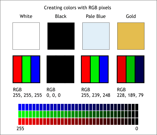
Numerically speaking, RGB images are 3D matrices with shape: Width: columns| Height: rows| Depth: 3
The Height and Width give us the number of pixels in each dimension. More pixels in each each dimension give us a larger picture or higher resolution (pixels per inch).
The Depth of 3 gives us three 2D matrices to store the color brightness values for each color (Red, Green, Blue) at each pixel. The values can take any value from 0 to 255, and their combinations result in over 16-million colors.
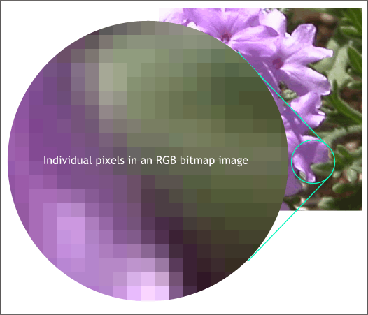
Here's an example of an RGB Photo zoomed in to the pixel level
| RGB Image Pixels | RGB Pixels as Integer Values |
|---|---|
 |
 |
Now that we know a little about RGB values, it's time to process the pictures! (Script here)
I wanted to eliminate color as a variable in order to give the classifier an easier task - identify shape or shading. To do that I used PIL's "L" algorithm to convert each image to grayscale (0-255) and de facto provide us with a 2D matrix.
Greyscaling Using PIL's 'L' Algorithm
Gray = R * 299/1000 + G * 587/1000 + B * 114/1000
Grayscale makes me smile. I hope it makes you smile too, because there are a lot of grayscale picture from here out!
Converting to grayscale allows us to do a couple things:
- Simplify the classification to shape and lighting only
- Maintain some semblance of sampling density (RGB features at 33px = 3267)
Once grayscaled, the images were resized to a fixed image size (33x33px). Creating a fixed image size keeps the pixel space consistent at 1089 total pixels.
I picked the image size by visually testing smallest picture size at which my human eye could accurately identify a "fish" or "non-fish".
| Fish Image Processing | Non-fish Image Processing |
|---|---|
 |
 |
Logistic Regression takes a 2D matrix as input, so each Image was flattened to a vector of length 1089 (33x33).
With all images converted to a 2D array, we can start to explore each class and their features.
Below is a plot that shows the mean of all pixels for both classes.
On the left, the mean "fish" appears to be of lower intensity on the borders with a brighter shading in the middle. If you squint, it might even look like a underwater photo of a fish.
On the right, the mean "Non-fish" picture appears to have a white border with some object of focus located directly in the center. Google Images seems to favor stock photos (objects on white background) for the first several images in a query. The webscraping script queried 200 words and pulled 5-6 images for each. As you can see, we have a large amount of stock photos in the "Non-Fish" class..
Let's take a look at the distribution of values for a random pixel. Pixel 496 is about halfway down the picture and 1 pixel in from the left.
The upper right and left plots are the "average" pictures from before. On the bottom is the Kernel Density Estimation (KDE) for both classes at pixel 496. Here we can see the probability distribution of this pixel and the Expected Value (mean) at that pixel.
Now in English: At pixel 496, "Fish" images have an expected intensity of ~110 (gray) and we can see the mode takes a value of ~90. "Non-fish" images at this pixel have an expected intensity closer to 190 (light-gray) with the mode at ~250.
The probability of an image being labeled "fish" will decrease as intensity increases above the combined mean at Pixel 496.
What does it look like if we subtract the means from each other to find the biggest difference in intensity? E.g. at Pixel 496, the difference between the classes is (~80).

Once we net the images at each pixel, we can normalize and rescale them back to 0-255 for image rendering.
Below we can see the biggest differences between the two images are at the edges.
On the right, I've applied a binary mask at the median (gray-128) to see exactly which pixels will give the classifier the strongest signal.

Now that we see where the classifier will be getting the strongest signal, let's visualize this across the pixel space. Watch where the dotted "Expected Value" lines get farthest apart.
To classify the pictures, I'm using classic Logistic Regression. Logistic Regression is similar to Linear Regression: modeling a dependent variable response to the change in independent variables.
Here's the big difference: While Linear Regression models a continuous output to continuous input:
Logistic Regression models the "Log Odds" (1.0-0.0) as output to continuous input:
This gives us a probability classification for two classes: "Fish" or "Non-Fish" in this case.
Since the feature space is so large (1089) relative to the sample size, I used an L1 regularization to penalize the model on the absolute value of the coefficients. This incentivizes the model to use the strongest features and eliminate non-contributing coefficients. I also scaled and standardized the data (For all columns, subtract the mean and divide by the standard deviation) to make the coefficients more stable and interpretable.
The interpretation of the coefficients is similar to that of linear regression. In this case, when the coefficient of a given pixel is positive, the probability of that image being a "fish" increases as pixel intensity increases. The opposite is also true.
Let's look at where the coefficients are positive and negative. (White = +, Black = -)
When we look at the Average Picture for each class we see that "Non-Fish" are generally brighter at the edges, while "Fish" pictures are brighter in the center. The direction of the coefficients speak to this relationship: As pixel intensity increases around the edges, we generally see a negative value for it's relative "fishiness". Conversely, in the middle, we see some positive correlation with pixel intensity and "fishiness".
Of note: Though the "Non-Fish" images were generally brighter at the edges, the positive coefficients at the top edge correspond to the few areas where the "Fish" images had a higher pixel intensity than the "Non-Fish" images.
For a more in-depth explanation on Logistic Regression, check out this article and the wiki.
Now that we've explored the data and the model, let's look at the results!
| ROC & AUC | Confusion Matrix |
|---|---|
 |
 |
Not bad! On the left, we see that the classifier achieved an Area Under the Curve of almost 78%. It was able to catch 71% of "Fish" pictures and 77% on "Non-Fish" pictures from a holdout set of 500 pictures that it had not previously seen.
Let's look at the archetypical samples from each class.
The "fishiest fish" is an image with a bright center and dark border, and the opposite is true for the "non-fish".
And just to make sure we haven't accidentally discovered the secret fish-detection powers of Logistic Regression.....
Going forward, I would like to build an image-classification neural net and app so that my friends can classify fish species.
Here are a few things I'll need to do:
- Get a list of fish species in Colorado
- Download at least 500 photos for each species of fish to classify
- Retrain a MobileNet classifier to classify fish species
- Train it better, or make a new model so it classifies accurately
- Make an app somehow
You can follow me on twitter or just email me.
List of people that I would like to thank:
- Jamie Sloat for her endless support.
- Rob Troup for his endless stream of great data science ideas.
- Frank Burkholder for great graphic ideas.
- Michael Dyer for tech geekery and tech support.
- Kelly Lutz for hyperlink help on the README
Copyright © 2018 Joe Shull


