Reservoir Computers and Chaotic Systems

This package contains an ode based reservoir computer for learning time series data. The package also includes functions for generating and plotting time series data for three chaotic systems.

Installation

The package is hosted on PyPi and can be installed with pip:

pip install rescomp

Alternatively, users can download the repository and add the location of the repo to their Python path.

Import the package with import rescomp as rc

Chaotic Systems

Currently, we support code to generate time series on three chaotic attractors. Time series can be generated with the orbit function and plotted in 3D with plot3d or in 2D with plot2d. (Plots are displayed in a random color so call the plot function again or supply color(s) to the keyword argument if it looks bad.)

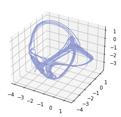
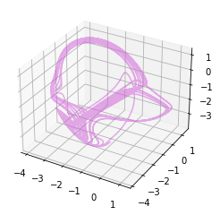
1. Thomas' cyclically symmetric attractor

t, U = rc.orbit("thomas", duration=1000, dt=0.1)
fig = rc.plot3d(U)

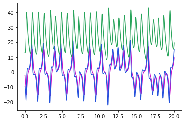
2. The Rossler attractor

t, U = rc.orbit("rossler", duration=100, dt=0.01)
fig = rc.plot3d(U)

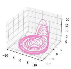
3. The Lorenz attractor

t, U = rc.orbit("lorenz", duration=100, dt=0.01)
fig = rc.plot3d(U)

Reservoir Computer Class

The package contains two options for reservoir computers: ResComp and DrivenResComp. The driven reservoir computers are still in beta stage but can be used for designing control algorithms [1]. Here is an example of learning and predicting Thomas' cyclically symetric attractor:

Train and Test

The train_test_orbit function returns training and testing sequences on the attractor. The test sequence immidiately follows the training sequence.

tr, Utr, ts, Uts = rc.train_test_orbit("thomas", duration=1000, dt=0.1)

Initialize the default reservoir computer and train on the test data with:

rcomp_default = rc.ResComp()
rcomp_default.train(tr, Utr)

Take the final state of the reservoir nodes and allow it to continue to evolve to predict what happens next.

r0 = rcomp_default.r0
pre = rcomp_default.predict(ts, r0=r0)
fig = rc.plot3d(pre)

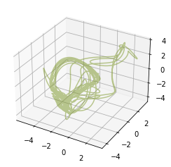
This doesn't look much like Thomas' attractor, suggesting that these parameters are not optimal.

Reservoir Hyperparameters

Optimized hyper parameters for each system are included in the package. Initialize a reservoir with optimized hyper parameters as follows:

hyper_parameters = rc.SYSTEMS["thomas"]["rcomp_params"]
rcomp = rc.ResComp(**hyper_parameters)

Train and predict as before.

rcomp.train(tr, Utr)
r0 = rcomp.r0
pre = rcomp.predict(ts, r0=r0)
fig = rc.plot3d(pre)

This prediction looks much more like Thomas' attractor.

Conclusion

Most high level functions are well documented in the source code and should describe the variables clearly. Good luck!

[1] Griffith, A., Pomerance, A., Gauthier, D.. Forecasting Chaotic Systems with Very Low Connectivity Reservoir Computers (2019)