hebtools - Time series analysis tools for wave data

This python package processes raw Datawell Waverider files into a flexible time series. The code allows easier calculation of statistics from the displacement data, more sophisticated masking of improbable data and the ability to deal with larger timeseries than is available from existing software. Similar code is also used to process pressure data from Nortek AWAC sensors details are described below.

The code is organised into one main package named hebtools with four subpackages awac, common, dwr and test

dwr

In the case of a Datawell Waverider buoy the buoy data directory containing year subfolders must be passed to the load method of the parse_raw module which then iterates through the years. Below is some example code ( from an IPython terminal session with comments interspersed ) for parsing the example data, then interrogating the files produced from the process:

Below is come code to parse a specific month, only the first path parameter is required, there is some example waverider data in the hebtools/data folder

In [1]: from hebtools.dwr import parse_raw 

In [2]: parse_raw.load("path_to_buoy_folder", year=2005, month="July", 
                       hdf_file_name='buoy_data.h5', calc_wave_stats=True)

The previous command will create a blosc compressed hdf5 file in the same directory as the raw files for that month, this can be inspected with the following command:

In [3]: import pandas as pd

In [4]: pd.HDFStore('path_to_buoy_folder/2005/July/buoy_data.h5')
Out[4]: 
<class 'pandas.io.pytables.HDFStore'>
File path: path_to_buoy_folder/2005/July/buoy_data.h5
/displacements            frame        (shape->[110557,11])                                     
/wave_height              frame_table  (typ->appendable,nrows->10599,ncols->4,indexers->[index])

The syntax below can be used to extract a specific frame as a DataFrame into pandas and read the first line of the dataframe.

In [5]: displacements_df = pd.read_hdf('path_to_buoy_folder/2005/July/buoy_data.h5',
                                      'displacements')

In [6]: displacements_df.head(1)
Out[6]:     sig_qual  heave  north  west                   file_name  extrema \ 
2005-07-01         0    -67    -37  -108  buoy}2005-07-01T00h00Z.raw      NaN   
           signal_error  heave_file_std  north_file_std  west_file_std \
2005-07-01        False       81.295838        52.67221      81.435775   
            max_std_factor  
2005-07-01        1.326198  

To understand what time period the DataFrame covers we can examine the index

In [7]: displacements_df.index
Out[7]:
<class 'pandas.tseries.index.DatetimeIndex'>
[2005-07-01 00:00:00, ..., 2005-07-01 23:59:59.200000]
Length: 110557, Freq: None, Timezone: None

To query specific columns in the DataFrame you can pass a list of column names via the [] syntax and additionally plot these columns as shown below.

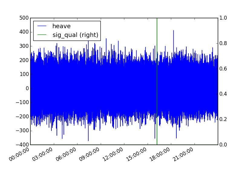
In [8]: displacements_df[['heave','sig_qual']].plot(secondary_y=('sig_qual'))
Out[8]: <matplotlib.axes._subplots.AxesSubplot at 0x1ff62470>

Plot will appear in separate window from IPython terminal ( see example below ).

It is possible to select a subset of a DatetimeIndexed DataFrame using the python datetime module as shown below.

In [9]: from datetime import datetime

In [10]: displacements_subset = displacements_df.ix[datetime(2005,7,1,16):datetime(2005,7,1,16,30)]

In [11]: displacements_subset.heave.plot(title='Heave data in centimetres', legend='heave')
Out[11]: <matplotlib.axes._subplots.AxesSubplot at 0x141e24e0>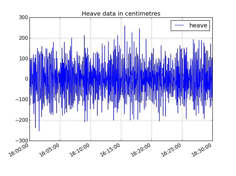

To get an overall idea of the data in the DataFrame you can use the describe function to return the maximum, minimum, mean and other parameters shown below.

In [12]: wave_heights_df = pd.read_hdf('path_to_buoy_folder/2005/July/buoy_data.h5','wave_height')
Out[12]: wave_heights_df.describe()
       wave_height_cm        period  max_std_factor
count    10599.000000  10599.000000    10599.000000
mean       211.435230      8.150750        2.025937
std         92.510379      2.625793        0.577351
min          6.000000      3.100000        0.400580
25%        142.000000      6.200000        1.608665
50%        205.000000      7.800000        1.978814
75%        271.000000     10.100000        2.380375
max        716.000000     19.600000        6.178612

To find out the particular record with a specific value we can pass a comparison into the ix function. The example below is to locate the timestamp for the maximum wave height. Measured from peak to trough.

In [13]: wave_heights_df.ix[wave_heights_df.wave_height.cm==wave_heights_df.wave_height_cm.max()]
Out[13]:                             
                            wave_height_cm  period \ 
2005-07-01 07:25:11.700000             716     8.6   

                                             file_name  max_std_factor  
2005-07-01 07:25:11.700000  buoy}2005-07-01T07h00Z.raw        4.390276 

To exclude certain results from the returned DataFrame we can again use the ix function and pass a less than or more than operator. The example below uses the max_std_factor column which is calculated by a comparison between the displacments for that record and the standard deviation for that 30 minute file.

In [14]: filtered_wave_heights = wave_height_df.ix[wave_height_df.max_std_factor<4]
Out[14]: filtered_wave_heights.describe()
       wave_height_cm       period  max_std_factor
count    10576.000000  10576.00000    10576.000000
mean       210.980333      8.15017        2.020694
std         91.780120      2.62615        0.566491
min          6.000000      3.10000        0.400580
25%        142.000000      6.20000        1.608198
50%        205.000000      7.80000        1.977909
75%        271.000000     10.10000        2.377813
max        572.000000     19.60000        3.998282

We can see that the overall number of records has reduced in this filtered DataFrame and the maximum wave height is now 572cm down from 716cm. We can also make comparisons between the two DataFrames, the example below shows the number of records filtered and how to return those records which have been filtered.

In [15]: len(wave_heights_df) - len(filtered_wave_heights)
Out[15]: 23

In [16]: filtered_wave_heights = wave_heights_df.ix[wave_heights_df.index.diff(filtered_wave_heights.index)]

We can also customise the plots, attaching labels to the axes by making use of the matplotlib package pyplot, as shown below plotting the wave heights of the filtered records as points, to see distribution over time and height:

In [17]: import matplotlib.pyplot as plt

In [18]: plt.figure()
Out[18]: <matplotlib.figure.Figure at 0x22995128>

In [19]: filtered_wave_heights.wave_height_cm.plot(style='.', markersize=10, title='Filtered Wave Records')
Out[19]: <matplotlib.axes._subplots.AxesSubplot at 0x22fe7780>

In [20]: plt.ylabel('Wave Heights in Centimetres')
Out[20]: <matplotlib.text.Text at 0x22ff0c50>

The module then processes the records from the raw files into a pandas DataFrame a good format for doing time series analysis. The main output is a DataFrame called displacements which includes the data from the raw files and extra columns which have been derived from the raw files, a smaller optional wave_heights dataframe is also produced providing details on individual waves extracted from the displacements. These dataframes are saved to an hdf5 file called buoy_data.h5 in the month folder using PyTables and the Blosc compression library.

Interrogating these output files in the DataFrame format requires a little knowledge of the pandas data structures and functionality. For example queries and plots inline from a real dataset see this example IPython Notebook An optional year and month parameter can be supplied to process a specific year, month folder. For more details on the approach taken to process the files please see the wiki

Masking and calculation of the standard deviation of displacement values takes place in the error_check module.

The parse_historical module takes a path to a buoy data directory ( organised in year and month subfolders ) and produces a joined DataFrame using the his ( 30 minute ) and hiw files stored in the month folders.

awac

In the awac package there is a parse_wad class that can process a Nortek AWAC wad file. The pressure column can be then be processed in the same way as the Waverider heave displacement without the error correction. The awac_stats.py module which uses an approach similar to wave_concat for calculating time interval based statistics.

parse_wap module takes a Nortek wave parameter file and generates a time indexed pandas Dataframe, with the optional name parameter if the produced DataFrame is intended to be joined to other data.

common

Peak and troughs are detected for the heave/pressure values in the GetExtrema class. In the WaveStats class wave heights and zero crossing periods are calculated, wave heights are calculated from peak to trough. The wave_power module

Testing

The test_dwr module for testing the parse_raw module and WaveStats class, example buoy data is required to test, one of day of anonymised data is provided in the data folder of the test package.

test_awac module tests the parse_wad and parse_wap modules. Short anonymised test data sets for wap and wad files are in the test folder.

Statistic outputs

The dwr/wave_concat module can be run after parse_raw to create a complete dataframe of all wave heights timestamped and sorted temporally for each buoy. The module uses data from the monthly wave_height_dataframe files, statistics are then calculated on the wave sets and then exported as an Excel workbook ( .xlsx file ). This module needs to be passed a path to a buoy data directory, the set size used for statistic calculation are based upon on the duration of the raw files ( usually 30 minutes ).

Statistical terms are calculated (Hrms,Hstd,Hmean where H is the wave heights ) and compared to the standard deviation of the heave displacement ( Hv_std ) to check that the waves conform to accepted statistical distributions.

Plot of output

The plot above compares wave height against the wave height divided by the standard deviation of the displacement signal, any values above 4 are considered to be statistically unrealistic for linear wave theory.

Background

The project was developed with data received from Waverider MKII and MKIII buoys with RFBuoy v2.1.27 producing the raw files. The AWAC was a 1MHz device and Storm v1.14 produced the wad files. The code was developed with the assistance of the Hebridean Marine Energy Futures and MERIKA projects.

Some more information on the data acquisition and overall workflow can be found on this poster

Requires:

• Python 2.7 ( developed and tested with 2.7.6 )
• numpy ( developed and tested with 1.6.2 )
• pandas ( minimum 0.12.0 )
• matplotlib ( developed and tested with 1.2.0 )
• openpyxl ( developed and tested with 1.6.1 )
• PyTables ( developed and tested with 3.0.0 )

All of the above requirements can be satisfied with a Python distribution like Anaconda, those that aren't installed by default can be installed via 'conda install package_name'.

Recommended optional dependencies for speed are numexpr and bottleneck, Windows binaries for these packages are available from Christoph Gohlke's page