Model-structured neural network framework for the modeling and control of physical systems

Modeling, control, and estimation of physical systems are fundamental to a wide range of engineering applications. However, integrating data-driven methods like neural networks into these domains presents significant challenges, particularly when it comes to embedding prior domain knowledge into traditional deep learning frameworks. To bridge this gap, we introduce nnodely (where "nn" can be read as "m," forming Modely), an innovative framework that facilitates the creation and deployment of Model-Structured Neural Networks (MSNNs). MSNNs merge the flexibility of neural networks with structures grounded in physical principles and control theory, providing a powerful tool for representing and managing complex physical systems. Moreover, a MSNN thanks to the reduced number of parameters needs fewer data for training and can be used in real-time applications.

Why use nnodely

The framework's goal is to allow the users fast modeling and control of a any mechanical systems using a hybrind approach between neural networks and physical models.

The main motivation of the framework are to:

• Modeling, control and estimation of physical systems, whose internal dynamics may be partially unknown;
• Speed-up the development of MSNN, which is complex to design using standard deep-learning framework;
• Support professionals with classical modeling backgrounds, such as physicists and engineers, in using data-driven approaches (but embedding knowledge inside) to address their challenges;
• A repository of incremental know-how that effectively collects approaches with the same purpose, i.e. building an increasingly advanced library of MSNNs for various applications.

The nnodely framework guides users through six structured phases to model and control physical systems using neural networks. It begins with Neural Models Definition, where the architecture of the MSNNs are specified. Next is Dataset Creation, preparing the data needed for training and validation. In Neural Models Composition, models are integrated to represent complex systems also including a controller if is needed. Neural Models Training follows, optimizing parameters to ensure accurate representation of the target system or a part of it. In Neural Model Validation, the trained models are tested for reliability. Finally, Network Export enables the deployment of validated models into practical applications. nnodely support a Pytorch (nnodely independent) and ONNX export.

Table of Contents

1. Getting Started
2. Basic Functionalities
   • Build the structured neural model
   • Neuralize the structured neural model
   • Load the dataset
   • Train the structured neural network
   • Test the structured neural model
3. Structure of the Folders
   • nnodely folder
   • tests folder
   • examples folder
4. License

Getting Started

You can install the nnodely framework from PyPI via:

pip install nnodely

Applications and use cases

The application of nnodely in some additional use cases are shown in https://github.com/tonegas/nnodely-applications.

How to contribute to the project

Download the source code and install the dependencies using the following commands:

git clone [email protected]:tonegas/nnodely.git
pip install -r requirements.txt

Give your contribution, open a pull request...

Or create an issue...

(back to top)

Basic Example

Build the neural model

The neural model, is based of a model-structured neural network, and is defined by a list of inputs by a list of outputs and by a list of relationships that link the inputs to the outputs.

Let's assume we want to model one of the best-known linear mechanical systems, the mass-spring-damper system.

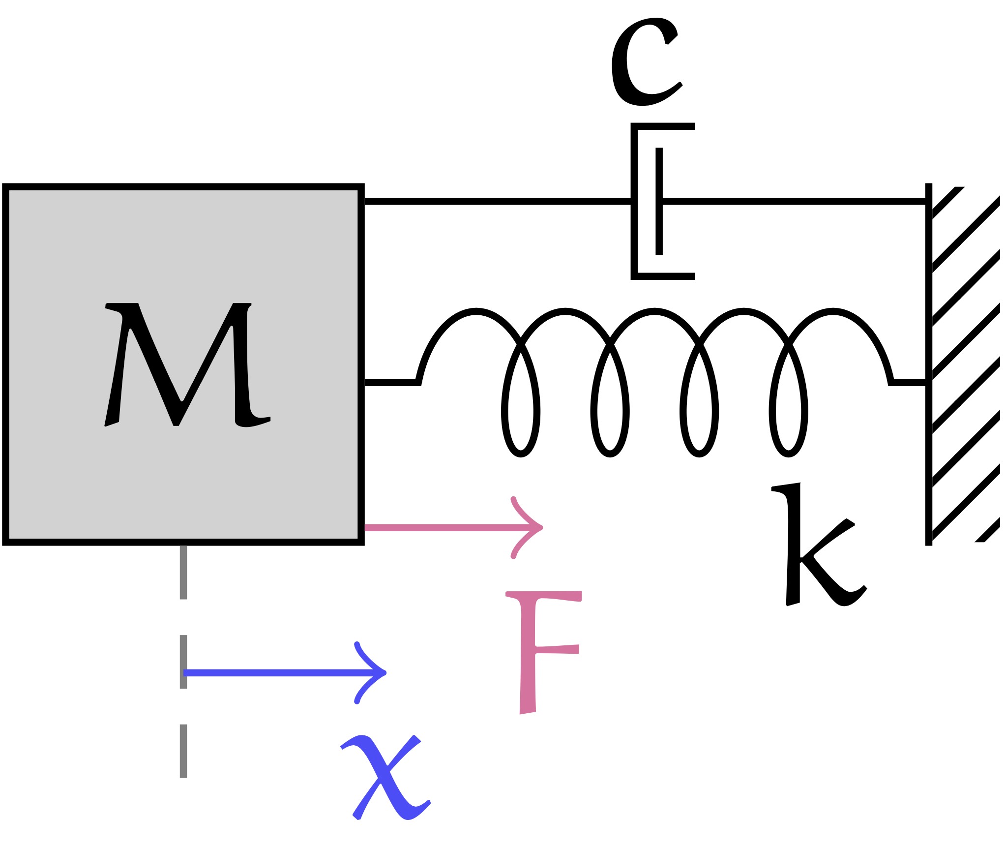
The system is defined as the following equation:

$$M \ddot x = - k x - c \dot x + F$$

Suppose we want to estimate the value of the future position of the mass given the initial position and the external force.

In the nnodely framework we can build an estimator in this form:

x = Input('x')
F = Input('F')
x_z_est = Output('x_z_est', Fir(x.tw(1))+Fir(F.last()))

The first thing we define the input variable of the system. Input variabiles can be created using the Input function. In our system we have two inputs the position of the mass, x, and the external force, F, exerted on the mass. The Output function is used to define an output of our model. The Output gets two inputs, the first is the name of the output and the second is the structure of the estimator.

Let's explain some of the functions used:

1. The tw(...) function is used to extract a time window from a signal. In particular we extract a time window of 1 second.
2. The last() function that is used to get the last force applied to the mass.
3. The Fir(...) function to build an FIR filter with the tunable parameters on our input variable.

So we are creating an estimator for the variable x at the instant following the observation (the future position of the mass) by building an observer that has a mathematical structure equal to the one shown below:

$$x[1] = \sum_{k=0}^{N_x-1} x[-k]\cdot h_x[(N_x-1)-k] + F[0]\cdot h_F$$

Where the variables $N_x$, and $h_f$ also the values of the vectors $h_x$ are still unknowns. Regarding $N_x$, we know that the window lasts one second but we do not know how many samples it corresponds to and this depends on the discretization interval. The formulation above is equivalent to the formulation of the discrete time response of the system if we choose $N_x = 3$ and $h_x$ equal to the characteristic polynomial and $h_f = T^2/M$ (with $T$ sample time). Our formulation is more general and can take into account the noise of the measured variable using a bigger time window. The estimator can also be seen as the composition of the force contributions due to the position and velocity of the mass plus the contribution of external forces.

Neuralize the structured neural model

Let's now try to train our observer using the data we have. We perform:

mass_spring_damper = Modely()
mass_spring_damper.addModel('x_z_est', x_z_est)
mass_spring_damper.addMinimize('next-pos', x.z(-1), x_z_est, 'mse')
mass_spring_damper.neuralizeModel(0.2)

Let's create a nnodely object, and add one output to the network using the addModel function. This function is needed for create an output on the model. In this example it is not mandatory because the same output is added also to the minimizeError function. In order to train our model/estimator the function addMinimize is used to add a loss function to the list of losses. This function takes:

1. The name of the error, it is presented in the results and during the training.
2. The second and third inputs are the variable that will be minimized, the order is not important.
3. The minimization function used, in this case 'mse'. In the function addMinimize is used the z(-1) function. This function get from the dataset the future value of a variable (in our case the position of the mass), the next instant, using the Z-transform notation, z(-1) is equivalent to next() function. The function z(...) method can be used on an Input variable to get a time shifted value.

The obective of the minimization is to reduce the error between x_z that represent one sample of the next position of the mass get from the dataset and x_z_est is one sample of the output of our estimator. The matematical formulation is as follow:

$$\frac{1}{n} \sum_{i=0}^{n} (x_{z_i} - x_{{z\_est}_i})^2$$

where n represents the number of sample in the dataset.

Finally the function neuralizeModel is used to perform the discretization. The parameter of the function is the sampling time and it will be chosen based on the data we have available.

Load the dataset

data_struct = ['time','x','dx','F']
data_folder = './tutorials/datasets/mass-spring-damper/data/'
mass_spring_damper.loadData(name='mass_spring_dataset', source=data_folder, format=data_struct, delimiter=';')

Finally, the dataset is loaded. nnodely loads all the files that are in a source folder.

Train the structured neural network

Using the dataset created the training is performed on the model.

mass_spring_damper.trainModel()

Test the structured neural model

In order to test the results we need to create a input, in this case is defined by:

1. x with 5 sample because the sample time is 0.2 and the window of xis 1 second.
2. F is one sample because only the last sample is needed.

sample = {'F':[0.5], 'x':[0.25, 0.26, 0.27, 0.28, 0.29]}
results = mass_spring_damper(sample)
print(results)

The result variable is structured as follow:

>> {'x_z_est':[0.4]}

The value represents the output of our estimator (means the next position of the mass) and is close as possible to x.next() get from the dataset. The network can be tested also using a bigger time window

sample = {'F':[0.5, 0.6], 'x':[0.25, 0.26, 0.27, 0.28, 0.29, 0.30]}
results = mass_spring_damper(sample)
print(results)

The value of x is build using a moving time window. The result variable is structured as follow:

>> {'x_z_est':[0.4, 0.42]}

The same output can be generated calling the network using the flag sampled=True in this way:

sample = {'F':[[0.5],[0.6]], 'x':[[0.25, 0.26, 0.27, 0.28, 0.29],[0.26, 0.27, 0.28, 0.29, 0.30]]}
results = mass_spring_damper(sample,sampled=True)
print(results)

(back to top)

Structure of the Repository

nnodely folder

This folder contains all the nnodely library files, the main files are the following:

1. activation.py this file contains all the activation functions.
2. arithmetic.py this file contains the aritmetic functions as: +, -, /, *., **,
3. fir.py this file contains the finite inpulse response filter function. It is a linear operation without bias on the second dimension.
4. fuzzify.py contains the operation for the fuzzification of a variable, commonly used in the local model as activation function.
5. input.py contains the Input class used for create an input for the network.
6. linear.py this file contains the linear function. Typical Linear operation W*x+b operated on the third dimension.
7. localmodel.py this file contains the logic for build a local model.
8. ouptut.py contains the Output class used for create an output for the network.
9. parameter.py contains the logic for create a generic parameters
10. parametricfunction.py are the user custom function. The function can use the pytorch syntax.
11. part.py are used for selecting part of the data.
12. trigonometric.py this file contains all the trigonometric functions.
13. nnodely.py the main file for create the structured network
14. model.py containts the pytorch template model for the structured network

Tests Folder

This folder contains the unittest of the library in particular each file test a specific functionality.

Examples of usage Folder

The files in the examples folder are a collection of the functionality of the library. Each file present in deep a specific functionality or function of the framework. This folder is useful to understand the flexibility and capability of the framework.

(back to top)

License

This project is released under the license License: MIT.

(back to top)